Debugging
One of the new features I could have utilized this time, thanks to the programming SWD interface, was using the mEDBG programmer and Atmel Studio 6.2 for debugging the code as I was writing it.

Atmel Toolchain\ARM GCC\Native\4.8.1443\CMSIS_Atmel\Device\ATMEL\saml21\
This was to update all the Studio's scripts and dependencies since I was working with Atmel Studio 6.2 which originally supported only pre-production versions (A) of the target MCU while the TT7B tracker ran on SAML21E17B microcontroller. I then went on to modify these files:
Atmel Studio 6.2\Devices\ATSAMD10D14AM.xml
Atmel Toolchain\ARM GCC\Native\4.8.1443\Resources\SamDeviceNameToHeaderMapping.xml
Atmel Toolchain\ARM GCC\Native\4.8.1443\CMSIS_Atmel\Device\ATMEL\saml21\include\sam.h
Atmel Toolchain\ARM GCC\Native\4.8.1443\CMSIS_Atmel\Device\ATMEL\saml21\include\saml21.h
The links contain the already modified versions of the files for download. The bottom three files contain only small changes. Mostly just altering paths of the ATSAMD10D14AM device. The contents of the first, however, were almost entirely replaced with the contents of ATSAML21E17B.atdf file from the downloaded pack.


| Clock | I [μA] | V [V] | P [μW] |
|---|---|---|---|
| OSC16M - 4MHz | 279 | 1.5 | 419 |
| OSC16M - 8MHz | 477 | 1.5 | 716 |
| OSC16M - 12MHz | 669 | 1.5 | 1004 |
| OSC16M - 16MHz | 834 | 1.5 | 1251 |
| OSC32K - 32kHz | 75 | 1.5 | 113 |
| XOSC32K - 32kHz | 74 | 1.5 | 111 |
| DFLL48M - 48MHz | 1413 | 1.5 | 2120 |
| FDPLL96M - 48MHz | 1414 | 1.5 | 2121 |
| XOSC32K - Standby | 9 | 1.5 | 14 |
I used this piece of code and its variations to check a number of possible ways to clock the microcontroller. The table above summarizes the power consumption of the whole TT7B board running on the specific clock source at a specific frequency. The board was detached from the debugger and supplied from a 1.5V LDO at its battery input port during the measurements. The current flowing from the LDO to the board was measured with μCurrent in the microampere setting.


Firmware
Github repository
With the help of the debugging interface, I eventually wrote and tested a number of libraries to control various peripherals of the MCU and to provide the functionality I had envisioned in the original design. The complete firmware for TT7B tracker in its current state can be found in the link above.


Following WatchDog, I continued in coding several core libraries such as two oscillator controllers (OSC), a generic clock controller (GCLK) and a power manager (PM) which all conduct basic MCU operation. In general, the microcontroller requires a source of a clock signal to step through and execute the programmed instructions. This is where the oscillator controllers come in allowing to choose from a number of options such as external crystals, internal oscillators, or a high speed digital frequency locked loop (DFLL48M) and a fractional digital phase locked loop (FDPLL96M). These source clock signals can then be individually prescaled and distributed to specific peripherals via the generic clock controller. The GCLK provides up to 9 generators (the main clock, MCLK, sourcing GCLK[0]) each being able to utilize a different source and supply different peripherals of choice. Running the device at frequencies higher than 12MHz requires switching it to a higher consumption Performance Level 2 (PL2) control of which, along with various sleep modes, is in the hands of the power manager.
A peripheral such as an analog-to-digital converter (ADC), digital-to-analog converter (DAC), real-time counter (RTC), etc. is typically made operational by first selecting a source GCLK generator and enabling a peripheral channel (PCHCTRLx register) to provide the peripheral with a clock signal. Following that, registers in the peripheral's domain can be set up and the peripheral enabled by setting the enable bit in the peripheral's CTRLA register.
A consequence of the possibility to run parts of the MCU at different frequencies manifests itself in the need to synchronize some of the peripheral's core registers with the rest of the microcontroller when written. This is in practice done by an empty while loop repeatedly checking a specific bit in the peripheral's SYNCBUSY or STATUS registers until it is cleared or set. That provides the required delay before executing further instructions.
The TT7B board is divided into several domains that can be individually powered up or down as described in the tracker's design. The manipulation of the general purpose I/O pins mediating this enable/disable functionality is carried out by the I/O pin controller (PORT). In some cases, such as the ADC and DAC, a peripheral utilizes I/O pins to input or output a signal. In these instances, the control over said pins has to be given to the peripheral. This again is in competency of the I/O pin controller (PMUXEN bit in PINCFG register).
Transmitter
The transmitter utilizes the digital-to-analog converter (DAC), two timer counters (TC) 0 and 4, and the inter-integrated circuit (I2C) interface mode of the serial communication interface (SERCOM) peripheral. The actual initialization routines and register configurations for the IC are then gathered in a separate library - SI5351B. Since the operation of the transmitter is a little bit more complex, it is outlined in this section.


| Drive Strength | Vp-p [V] | P [mW] | P [dBm] |
|---|---|---|---|
| 2mA | 0.88 | 1.94 | 2.87 |
| 4mA | 1.64 | 6.72 | 8.27 |
| 6mA | 2.10 | 11.02 | 10.42 |
| 8mA | 2.70 | 18.22 | 12.61 |
The peak to peak voltages in the table differ from the voltages seen in the screengrabs as they varied a little in time, and I tried to use the mid values for the calculations.

| Drive Strength | P [mW] | P [dBm] |
|---|---|---|
| 2mA | 1.48 | 1.70 |
| 4mA | 5.25 | 7.20 |
| 6mA | 9.33 | 9.70 |
| 8mA | 12.49 | 10.97 |
This time the results were lower but at least in the same ballpark. Nevertheless, I wanted to know more and did the same measurements while transmitting 1MHz, 10MHz and 100MHz carrier waves subsequently.
| Drive Strength | P1 [mW] | P1 [dBm] | P10 [mW] | P10 [dBm] | P100 [mW] | P100 [dBm] |
|---|---|---|---|---|---|---|
| 2mA | 0.40 | -3.99 | 0.45 | -3.47 | 1.32 | 1.20 |
| 4mA | 0.78 | -1.07 | 1.58 | 2.00 | 4.79 | 6.80 |
| 6mA | 0.88 | -0.55 | 2.57 | 4.10 | 9.55 | 9.80 |
| 8mA | 0.92 | -0.38 | 3.16 | 5.00 | 13.66 | 11.35 |
The 100MHz results were more or less comparable to the initial 144MHz measurement, however the 1 and 10MHz carriers recorded much lower output power. Especially the 10MHz results being 6-7dB lower compared to the results produced by the first method were a bit confusing. In case of the 1MHz signal, lower output was expected due to the probable high-pass filtering mentioned earlier. Unfortunately, I don't have a high sample rate oscilloscope at hand, so I can't really probe the 144MHz signal and see how effective the designed low-pass filtering is.

On TT7B, the code initializes two timer counters, each for one tone - 1200Hz and 2200Hz. By running the timers at much higher frequencies, the code can step through lookup tables which contain values from 0 to 4095 that represent a single wavelength of a sine wave which are then fed to the 12-bit digital-to-analog converter. When timed right, the output of the DAC is a continuous sine wave of the desired frequency. As timing is critical, the stepping through tables and feeding the DAC is all done in the timer counter's interrupts. The interrupt managing the 1200Hz tone also takes care of the transmission's bit rate (switching between transmitting a '0' or a '1') since that is for APRS 1200bps as well.
I mentioned lookup tables in plural. That is because due to pre-emphasis the 1200Hz and 2200Hz tones should differ in amplitude. A quite detailed discussion on pre- and de-emphasis in APRS transmissions can be found here. I decided to avoid inflating the interrupt handlers with instructions recalculating the adjustments, and instead stored two lookup tables in RAM, one for each tone.


| Settings 1 | Settings 2 | Settings 3 | |
|---|---|---|---|
| REFCLK | XOSC32K | XOSC32K | XOSC32K |
| LDR | 2009 | 2009 | 1545 |
| LDRFRAC | 15 | 15 | 14 |
| FDPLL96M | 65,894,400Hz | 65,894,400Hz | 50,688,000Hz |
| GCLK[0].DIV | 4 | 2 | 2 |
| MCLK: GCLK[0] | 16,473,600Hz | 32,947,200Hz | 25,344,000Hz |
| GCLK[1].DIV | 16 | 6 | 12 |
| DAC: GCLK[1] | 4,118,400Hz | 10,982,400Hz | 4,224,000Hz |
| TC0.COUNT | 858 | 1716 | 660 |
| TC0 interrupt | 19,200Hz | 19,200Hz | 38,400Hz |
| TC4.COUNT | 468 | 936 | 360 |
| TC4 interrupt | 35,200Hz | 35,200Hz | 70,400Hz |
| Lookup 1200hz | 16 | 16 | 32 |
| Lookup 2200hz | 16 | 16 | 32 |
When working on the timing of the modulation, I tried a number of OSC/MCLK/TC setups out of which the three specific cases described in the table above were proven to work. The point was to find such a main clock frequency that would allow oversampling the 1200Hz and 2200Hz tones using only whole integer clock divisors and TC count values. The lower limit for main clock frequency was then determined by the length of the interrupt routines in terms of instructions. To produce the sine waves at desired frequencies, the microcontroller has to be able to execute the whole code within the two interrupts between individual timer counter's compare matches, and hence interrupt firings. For example, to produce the 2200Hz tone from a 16 element lookup table, the TC4's interrupt has to fire with a frequency of 16 * 2200Hz = 35,200Hz. That can be achieved by setting the timer to fire a compare match interrupt in 468 clock cycles provided the main clock runs at 35,200Hz * 468 = 16,473,600Hz. That at the same time means there are 468 clock cycles to execute whatever code is within the interrupt. To have the microcontroller operate at said frequency, the FDPLL96M can be setup to run at 65,894,400Hz using LDR and LDRFRAC values, representing the multiplier of a reference frequency, of 2009 and 15, respectively (equation in the datasheet). The reference itself is then set to be XOSC32K which on TT7B is a 32.768kHz TCXO. GCLK[0], which is the main clock, is set to source signal from the FDPLL96M and divides it by four. The operating frequency of the DAC (provided by GCLK[1]) is not that important. It just has to be fast enough to finish a conversion between individual lookup table steps.
To make this all work, I had to use two 16-bit timer counters, one for each tone. TC0, the main timer counter, is not only responsible for generating the 1200Hz tone, but also decides which bit, or rather which tone, to transmit now by enabling/disabling TC4's compare match interrupt responsible for the 2200Hz tone. In practice, proper timing of the next interrupt is achieved by adding a respective number of counts to the timer's COMPARE register (designated as TCx.COUNT in the table above).
| VCXO Pull | 0.0V | 0.913V | 1.826V | Bandwidth |
|---|---|---|---|---|
| 30ppm | -4344Hz | -1918Hz | 507Hz | 4851Hz |
| 38ppm | -5502Hz | -2430Hz | 643Hz | 6145Hz |
| 40ppm | -5792Hz | -2558Hz | 677Hz | 6469Hz |
| 50ppm | -7240Hz | -3197Hz | 846Hz | 8086Hz |
| 240ppm | -34752Hz | -15346Hz | 4060Hz | 38812Hz |
Si5351B allows setting the degree to which voltage present on its VC pin pulls the output frequency in parts-per-million. The selectable settings range from +-30ppm to +-240ppm. Since on TT7B the Si5351B operates at 3.3V (3.27V when measured on the actual board), and the microcontroller's DAC outputs voltages in range of 0V to 1.8V only (1.826V when measured on the board), just a portion of the pullable range will be available. Additionally, the midpoint of the modulation will be offset in frequency due to this as well. The table above shows calculated offsets from a programmed carrier frequency of 144.8MHz at a specific pull setting and DAC output voltages. I made a choice of 38 ppm pull for the actual transmissions which was based on desired peak deviation of 3.0kHz of the 2200Hz tone and 1.65kHz of the 1200Hz tone. More details on the peak deviations in APRS transmissions again in the previously link article. The 2200Hz lookup table ranges in values from 0 to 4095 (12-bit DAC) while the 1200Hz lookup table is appropriately scaled. When devising the offset for the programmed frequency, I had to take into account not only the value at 0.913V from the table above, but also include additional fixed offset which originated in the fact that this specific TT7B board was equipped with a VCXO version of the TCXO and its voltage control pin was tied to ground. According to the datasheet, that should pull its output frequency by -5ppm which would at 144.8MHz add further 724Hz to the total offset.
| Area | F [MHz] | FVCO [MHz] | Offset [Hz] |
|---|---|---|---|
| North America | 144.390 | 866.340 | -3920 |
| New Zealand | 144.575 | 867.450 | -3890 |
| S. Korea | 144.620 | 867.720 | -3880 |
| China | 144.640 | 867.840 | -3880 |
| Japan | 144.660 | 867.960 | -3885 |
| Europe, Russia | 144.800 | 868.800 | -3855 |
| Argentina, Uruguay | 144.930 | 869.580 | -3940 |
| Venezuela | 145.010 | 870.060 | -3920 |
| Australia | 145.175 | 871.050 | -3990 |
| Thailand | 145.525 | 873.150 | -3910 |
| Brazil | 145.570 | 873.420 | -3910 |
Prior to each transmission, the Si5351B is programmed to a specific frequency. For the sake of simplicity, the code focuses on programming the VCO frequency which is then always divided by an integer divider of 6 to get the desired output. This approach works fine for all 2m band APRS frequencies, but for any output below 100MHz the code would have to be modified. The last column in the table contains actual measured offsets of midpoints of modulation at individual APRS frequencies. They are several hundred hertz larger than the previously calculated values and slightly differ frequency to frequency. Since the differences aren't that large, a fixed offset of 3900Hz is automatically added when a new frequency is programmed to the Si5351B.


These are the actual recordings, the 16 element table with main clock at 16MHz at the top, and the 32 element table running at 25MHz at the bottom. Both .wav files can be downloaded here: 16 element and here: 32 element.

Encoding
As mentioned previously, the task of the tracker is to deliver back as much information about the balloon itself and its surrounding conditions as possible. For that, the tracker will use the worldwide APRS network of iGates and digipeaters. Although the APRS protocol supports sending telemetry along positional information and can even graph the data, the amount of data is limited. To send all the data I wanted, I decided to define my own packet structure, use the APRS network to only collect the data packets, and do the decoding manually. The position of the balloon will still be plotted online on a map such as aprs.fi, but all the telemetry data will be reported encoded in the comment section of the APRS packet.
| !/5LD\S*,yON2WYm%=,)ZiLx,f:-D33ZM0!<QU |
|---|
| !/5LD\S*,yON2WYm%=,)ZiLx,f:-D33ZM0!<QU5N^JS%<z!(Z/'T$r7U@#]KRj1F(!9T,wQ7,8Z |
|---|
An example of the packet TT7B will be sending can be seen above. The first is a shorter packet containing only current information, while the second is a full length packet containing current information and an additional backlog of data acquired previously during the flight. This is used to provide information about the balloon's whereabouts for when it was outside of reception range. The shorter packet is 38 bytes long plus additional 39 bytes of flags, paths and crc. The full length packet is 75 bytes plus again the additional 39 bytes. It takes 513ms in total to transmit the 77 bytes of the shorter packet, and 760ms to transmit the 114 byte packet.
| Byte | Symbol | Description | Decoded |
|---|---|---|---|
| 0 | ! | Data Type Identifier | |
| 1 | / | Symbol Table Identifier | |
| 2:5 | 5LD\ | Latitude | 49.49148° |
| 6:9 | S*,y | Longitude | 18.22311° |
| 10 | O | Symbol Code (Balloon) | |
| 11:12 | N2 | Altitude (coarse) | 1127.42m |
| 13 | W | Compression Type Identifier |
The first 14 bytes of the packet constitute a standardized compressed position report as described in APRS Protocol Reference 1.0.1. Latitude and longitude can be decoded using these equations: $$Latitude=90-((c_1-33)\times 91^3+(c_2-33)\times 91^2+(c_3-33)\times 91+(c_4-33))/380926$$ $$Longitude=-180+((c_1-33)\times 91^3+(c_2-33)\times 91^2+(c_3-33)\times 91+(c_4-33))/190463$$ where $c_{1..4}$ represent individual chars $5LD\setminus$ for latitude and $S*,y$ for longitude. Following the same char representation, altitude in meters can be decoded using this equation: $$Altitude=1.002^{(c_1-33)\times 91+(c_2-33)}/3.28084$$ The compression and decompression introduce some amount of error in the original values. In case of latitude, the resolution can be down to 29cm, while in case of longitude down to 59cm which corresponds to higher accuracy then most GPS modules can achieve. However in case of altitude, the potential error increases with the altitude itself. At 12,000m it can be up to 24m, at 40,000m it can be up to 80m. For this reason, there is additional correction data transmitted among the data in the remainder of the packet to report altitude data within 1m of the measured value. Note that these errors originate purely in the compression process and do not say anything about the accuracy of the positional fix itself.
| Byte | Symbol | Description | Decoded |
|---|---|---|---|
| 14:15 | Ym | Temperature MCU | 23.44°C |
| 16:17 | %= | Temperature THERMISTOR_1 | 23.74°C |
| 18:19 | ,) | Temperature THERMISTOR_2 | 0.01°C |
| 20:21 | Zi | Temperature MS5607_1 | 25.18°C |
| 22:23 | Lx | Temperature MS5607_2 | 0.00°C |
| 24:26 | ,f: | Pressure MS5607_1 | 97395Pa |
| 27:29 | -D3 | Pressure MS5607_2 | 102575Pa |
| 30:31 | 3Z | Battery Voltage | 1.512V |
| 32:33 | M0 | Ambient Light | 22.10lux |
| 34:37 | !<QU | Altitude (offset: 0-99m), Satellites, Active Time, Last Reset |
This portion of the packet contains the current telemetry data. All individual data points in some form utilize Base91 encoding to transform their original value to an ASCII character representation that is transmittable via APRS. The thermistor one and two temperatures, and battery voltage are all raw ADC readings (0-4095) Base91 encoded into two ASCII characters. The following equation is common to all of them: $$ADC_{raw}=(c_1-33)\cdot 91+(c_2-33)$$ After acquiring the raw ADC values, the calculations differ. To get the temperature measured by a thermistor in °C, first calculate the voltage the raw ADC value represents. This voltage is across the thermistor itself in a voltage divider setup and allows to calculate the thermistor's resistance. The resistance then plugs into a Steinhart-Hart equation where $R_2$ is the resistance at temperature $T_{therm}$. The coefficients $a$, $b$ and $c$ were determined earlier for this specific thermistor. $$V_{R2}=\frac{ADC_{raw}}{4095}\cdot 1.826V$$ $$R_{2}=\frac{V_{R2} \cdot 49900\Omega}{1.826V - V_{R2}}$$ $$T_{therm}=\frac{1}{0.00128424+0.00023629\cdot ln(R_{2})+0.0000000928\cdot ln(R_{2})^3}-273.15$$ The battery voltage in volts can be calculated by following this equation. The factor of 2 comes from the fact that the measurement is done after a voltage divider. $$V_{batt}=\frac{ADC_{raw}}{4095}\cdot 1.826V\cdot 2$$ The MCU and the two MS5607 temperature readings follow the same decoding process. First decode the Base91 encoded value $n$. Then subtract an offset of 4000 from $n$ and divide the result by 50 to get the actual temperature in °C. $$n=(c_1-33)\cdot 91+(c_2-33)$$ $$T=\frac{n-4000}{50}$$ In case of the two pressure values, all that needs to be done is to decode the three Base91 encoded characters. The result is a pressure value in Pa. $$P=(c_1-33)\cdot 91^2+(c_2-33)\cdot 91+(c_3-33)$$ The ambient light readings produced by the sensor can span from 0.0072 to 120,000lux. To preserve resolution at even the very low end of the range and not waste too many characters in transmitting these values, I decided to utilize a similar approach as is used in the original APRS format to compressed altitude. The consequential decrease in resolution at the higher end of the range of possible values doesn't matter that much here. The following equations result in an illuminance reading in lux. $$n=(c_1-33)\cdot 91+(c_2-33)$$ $$E_v=\frac{10^{n\cdot log(1.002)}}{139}$$ The last four characters of this section of the packet encode a few different values together. First decode the Base91 encoding to a single number. $$n=(c_1-33)\cdot 91^3 + (c_2-33)\cdot 91^2+(c_3-33)\cdot 91+(c_4-33)$$ Last Reset is a number between 0 and 5 corresponding to the source of the last reset as reported by the microcontroller in register RCAUSE. The sources are: 0 - NONE no reset source; 1 - POR power on reset; 2 - BOD brown out detector; 3 - EXT external; 4 - WDT watchdog timer; 5 - SYS system reset. To get the value use the following equation. $$reset=n\; mod\; 6$$ Active Time is the time measured by the onboard Real-Time Counter between waking up from standby mode to construction of the APRS packet, so the actual transmission of 0.5-0.7s is excluded. The point of this measurement is to get information on the time to first fix of the GPS module. The resolution is 0.1s. $$t=\bigg(\bigg\lfloor\frac{n}{6}\bigg\rfloor\; mod\;1000\bigg)/10$$ The next value to extract is the number of satellites used in the GPS positional fix. To get the number follow this equation. $$sats=\bigg(\bigg\lfloor\frac{n}{6\cdot 1000}\bigg\rfloor\; mod\;17\bigg)$$ As mentioned earlier, the compression and decompression used when transmitting altitude data introduces an error. To compensate for this error, Altitude Offset is added to Altitude Coarse rounded down to nearest integer. The following equation reveals how to arrive at the value. $$alt=\bigg\lfloor\frac{n}{6\cdot 1000\cdot 17}\bigg\rfloor$$ In this example !<QU decodes as: Last Reset = 1; Active Time = 0.1s; Satellites = 4; Altitude Offset = 2m which when added to Altitude Coarse gives an altitude of 1129m reported by the GPS module. This collective encoding is used in a couple of instances in the following backlog section as well.
| Byte | Symbol | Description | Decoded |
|---|---|---|---|
| 38:41 | 5N^J | Backlog: Latitude | 49.44184° |
| 42:45 | S%<z | Backlog: Longitude | 18.01337° |
| 46:49 | !(Z/ | Backlog: Altitude (precise: 0-50,000m), Satellites, Last Reset | |
| 50:54 | 'T$r7 | Backlog: Year, Month, Day, Hour, Minute, Active Time | |
| 55:56 | U@ | Backlog: Temperature MCU | 15.26°C |
| 57:58 | #] | Backlog: Temperature THERMISTOR_1 | 35.99°C |
| 59:60 | KR | Backlog: Temperature THERMISTOR_2 | -62.65°C |
| 61:62 | j1 | Backlog: Temperature MS5607_1 | 53.18°C |
| 63:64 | F( | Backlog: Temperature MS5607_2 | -12.52°C |
| 65:67 | !9T | Backlog: Pressure MS5607_1 | 2235Pa |
| 68:70 | ,wQ | Backlog: Pressure MS5607_2 | 98965Pa |
| 71:72 | 7, | Backlog: Battery Voltage | 1.795V |
| 73:74 | 8Z | Backlog: Ambient Light | 0.5279lux |
This last portion of the APRS packet contains the optional backlog. Most of the data such as latitude, longitude, MCU, thermistor and MS5607 temperatures, MS5607 pressure, battery voltage, and ambient light are encoded in the same way as in the current data section. The bytes 46 to 49 collectively represent encoded altitude (this time without encoding error), the number of satellites and information about the last reset source. The process once again starts with decoding the Base91 representation. $$n=(c_1-33)\cdot 91^3 + (c_2-33)\cdot 91^2+(c_3-33)\cdot 91+(c_4-33)$$ Extracting the Last Reset value follows the same steps as previously. $$reset=n\; mod\; 6$$ Getting the number of Satellites is slightly different to previously. $$sats=\bigg(\bigg\lfloor\frac{n}{6}\bigg\rfloor\; mod\;17\bigg)$$ And the precise Altitude is arrived at by following this equation. $$alt=\bigg\lfloor\frac{n}{6\cdot 17}\bigg\rfloor$$ In this example !(Z/ decodes as: Last Reset = 0; Satellites = 5; Altitude Precise = 619m.
The remaining bytes 50 to 54 collectively represent encoded year, month, day, hour, minute and active time of the backlogged telemetry. Since there are five Base91 encoded bytes this time, the first step is slightly different. $$n=(c_1-33)\cdot 91^4+(c_2-33)\cdot 91^3+(c_3-33)\cdot 91^2+(c_4-33)\cdot 91+(c_5-33)$$ First the Active Time is extracted in this way. $$t=\frac{n\; mod\; 1000}{10}$$ Followed by the Minute. $$min=\bigg(\bigg\lfloor\frac{n}{1000}\bigg\rfloor\; mod\;60\bigg)$$ Then the Hour. $$hour=\bigg(\bigg\lfloor\frac{n}{1000\cdot 60}\bigg\rfloor\; mod\;24\bigg)$$ And the Day. $$day=\bigg(\bigg\lfloor\frac{n}{1000\cdot 60\cdot 24}\bigg\rfloor\; mod\;31\bigg)+1$$ The Month. $$month=\bigg(\bigg\lfloor\frac{n}{1000\cdot 60\cdot 24\cdot 31}\bigg\rfloor\; mod\;12\bigg)+1$$ And lastly the Year. $$year=\bigg\lfloor\frac{n}{1000\cdot 60\cdot 24\cdot 31\cdot 12}\bigg\rfloor +2018$$ In this specific example 'T$r7 decodes as: Active Time = 12.3s; Minute = 34; Hour = 10; Day = 3; Month = 11; Year = 2018.


GPS
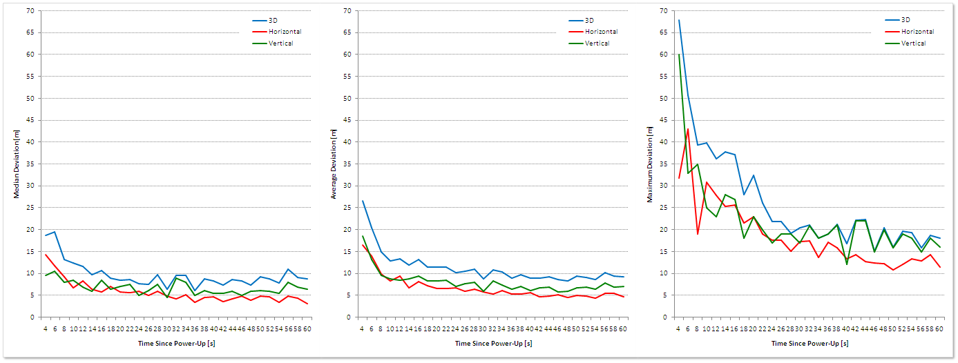
Since the GPS module is the most power hungry individual part on the tracker, the main goal was to find the right compromise between power consumption and positional accuracy of its measurements. The ZOE-M8B's datasheet states a horizontal position accuracy of 2.5m when the receiver is in Continuous mode, 3.0m when in Super-E Performance mode, and 3.5m in Super-E Power Save mode for positional solutions based on signals from the GPS constellation alone. The module can also utilize the GLONASS, BeiDou and Galileo GNSS systems, or their combination with less accuracy (according to the datasheet values) and more power consumed. The accuracy is stated in Circular Error Probable (CEP) figures specified over a 24 hour period with the receiver being locked on to 6 or more satellites at signal levels of -130dBm. The Continuous mode figure, for example, means that 50% of position measurements over the specified period were somewhere within a circle 2.5m in radius centered at the real position, while the remaining 50% lay an unspecified distance outside that circle. The datasheet didn't provide any figures on vertical accuracy.
It should be noted that these figures were achieved with ideal conditions as specified. Real life positional measurements are often scattered around a bit more depending on the actual environment. The typically mentioned sources of error are inaccuracies in satellite clock and orbit, deviations of the real conditions from the receiver's ionospheric and tropospheric models, the receiver measuring reflected signals instead of direct signals (multipath), or the actual geometry of the satellite constellation (often expressed as various Dilution Of Precision (DOP) values). The Essentials of Satellite Navigation document, which can be found on u-blox's website, discusses the matter in more detail and is a useful source of information on GPS operation in general. In case of doing accuracy tests in real life environments, the multipath error and the actual geometry of satellites used in the solution will most likely be the main variables compared to the ideal conditions case.


| Settings | 3Dmed | 3Davg | 3Dmax | Hmed | Havg | Hmax | Vmed | Vavg | Vmax |
|---|---|---|---|---|---|---|---|---|---|
| Super-E, GPS, GLONASS | 11.9m | 14.4m | 53.9m | 7.8m | 9.0m | 37.7m | 7.3m | 10.0m | 47.3m |
| Continuous, GPS | 6.6m | 7.4m | 27.7m | 3.1m | 3.7m | 16.9m | 5.4m | 5.9m | 24.4m |
| Continuous, GPS, GLONASS, Galileo | 7.8m | 9.3m | 38.0m | 4.8m | 5.3m | 25.3m | 5.6m | 7.0m | 33.6m |
| Continuous, GPS, SBAS | 4.6m | 5.1m | 29.5m | 2.6m | 2.8m | 11.9m | 3.2m | 3.8m | 27.2m |
| Continuous, GPS, 4 sats, standby | 27.5m | 33.2m | 294.3m | 17.6m | 22.6m | 226.5m | 14.2m | 20.5m | 187.8m |
| Continuous, GPS, 6 sats, standby | 23.3m | 28.0m | 113.8m | 12.2m | 14.4m | 72.6m | 16.3m | 22.0m | 109.3m |
| Continuous, GPS, 6 sats, 4Hz, standby | 17.6m | 20.1m | 91.0m | 9.4m | 10.5m | 43.2m | 12.3m | 15.5m | 83.3m |
| Continuous, GPS, 7 sats, 4Hz, standby | 18.6m | 21.4m | 67.2m | 9.9m | 11.2m | 45.0m | 13.1m | 16.6m | 62.1m |
This table summarizes the previous data in actual numbers. The median, average and maximum deviations in three-dimensions, horizontally and vertically are referenced to the average position of the dataset (marked by the white dot). Immediately, it is apparent that when the u-blox module is supplied continually and thus allowed to track and acquire satellites without interruptions, the accuracy is much better. The Super-E mode, which is a module controlled power saving operation, results in higher deviations than when the module runs full power in Continuous mode. Concerning GLONASS, Galileo and BeiDou, there is a further discussion on these constellations a little later. Having the module receive SBAS satellites improves the accuracy slightly, it is, however, unusable for discontinuous supply operation where the time to first valid fix is critical as the SBAS satellites require longer times to get incorporated in the positional solutions. When the module is regularly brought in and out of hardware backup mode by cutting and restoring the main supply, it every time undergoes a hot start during which it has to re-lock onto satellites. Provided the backup period is short enough (less than 4 hours), and the module is able to track time with an external RTC, it can use the time and previously acquired orbital data now stored in its battery backed RAM to quickly search much smaller frequency/timeshift space and re-synchronize with the known satellite signals. The table shows that waiting for a solution based on more satellite signals increases accuracy, though, it for some reason doesn't come close to accuracy of a continually supplied receiver.

| GNSS | Earth [dBW] | C/N0 [dBHz] | Cold [dBHz] | Hot [dBHz] | Track [dBHz] |
|---|---|---|---|---|---|
| GPS | -158.5 | 45.5 | 26.0 | 17.0 | 8.0 |
| GLONASS | -161.0 | 43.0 | 30.0 | 20.0 | 8.0 |
| BeiDou | -163.0 | 41.0 | 31.0 | 19.0 | 14.0 |
| Galileo | -157.0 | 47.0 | 36.0 | 23.0 | 15.0 |
By changing the settings in the UBX-CFG-GNSS message, I also tested GLONASS only, Galileo only, and BeiDou only reception. However, neither setting managed to get a valid fix in under 20 minutes. After a more detailed examination, I found that the UBX-NAV-SAT message never reported any GLONASS, Galileo, nor BeiDou satellites with 'acquired signal', only a few flagged as 'searching signal'. A web-based GNSS constellation viewer was showing plenty of satellites in the sky during that time. The table above summarizes minimum signal power levels in dBW expected at the surface of Earth for individual systems and corresponding Carrier to Noise ratios (C/N0) in dBHz at noise power density of -204dBW/Hz. The latter three columns then contain minimum signal levels needed during a receiver cold start, hot start, and tracking phases derived from the receiver's sensitivity values for continuous mode stated in the datasheet. Although, signal levels too close to the minimum values will lead to longer acquisition times as the probability of an error in decoding the navigation message increases. Values in the range of 32 to 36dBHz are typically mentioned for a reliable GPS navigation data acquisition. It is apparent from the table that the ZOE-M8B receiver is most suited for the GPS signals, while the other systems require better signal conditions. It is thus possible that the design of the PCB with a simple ceramic chip antenna on TT7B is not sufficient for the other constellations. At least not in the environment where I tested it.


In short, the previous findings can be summarized as less power consumed, less accurate measurements. Given the tracker will be battery powered and accuracy approaching the datasheet values comes only with prolonged active times, saving power will be prioritized at the cost of larger average deviations in the reported positions. Thus, I don't expect to be able to follow subtle variations in altitude very closely that could in principle be linked to variations in temperature and pressure measured be the other sensors. The actual control of the module will constitute having it receive only GPS satellites (and QZSS satellites as recommended in the datasheet), setting the measurement rate to 10Hz to shorten the active time, externally controlling the main power supply thus forcing the module to hardware backup mode, and switching the module to the Continuous mode to leave it in acquisition or tracking states during wake-up periods.
In terms of the code, the functions to enable or disable the main power supply to the u-blox module can be found in the PORT library operating the I/O Pin Controller. The communication between the MCU and the module is serviced by functions in another SERCOM library this time dedicated to the Universal Synchronous and Asynchronous Receiver and Transmitter (USART). The default baud rate the module expects is 9600 which can be increased to 115200 baud, for example. This shortens the transmission time of a 100 byte UBX-NAV-PVT message from 104ms to less than 9ms. All functions written to modify various settings, poll desired messages, and parse the received responses can be found in the ZOE_M8B library.
A centimeter positional accuracy is possible with GPS, however, it belongs to the scope of more advanced and expensive technologies. Differential GNSS (DGNSS, DGPS) techniques achieve higher accuracy by having a stationary reference receiver calculate and transmit corrections for the signals from individual satellites. These are then received and applied to measurements by mobile receivers. This approach is, however, limited by the required proximity to the reference station. Real Time Kinematics (RTK) further increases accuracy by employing carrier phase measurements on top of the base station-rover setup as opposed to just measurements of the slower pseudorandom code's chips. The NEO-M8P module by u-blox is one example that supports this functionality. Another technique that increases accuracy is employed in dual band receivers such as the ZED-F9P. These modules are able to correct for the ionosperic delay by receiving two different frequency signals from one satellite (L1C/A and L2C for example), and from the measured difference in arrival time correct the error caused by the ionosphere. In case of ZOE-M8B and TT7B, it is realistic to expect accuracy in ranges as detailed in the tests above, or potentially slightly improved by the unobstructed view of sky at altitude and the lack of multipath error under a balloon.
External Sensors
The MCU's temperature sensor, the ambient light sensor (VEML6030), and one pressure/temperature sensor (MS5607) were already populated on the tracker after reflow. The remaining sensors - the onboard thermistor, the external thermistor, and the external pressure/temperature sensor - had to be added separately.


Based on the performance of my previous superpressure balloons, the tracker is expected to operate at altitudes between 10,000 to 13,000 meters. This range corresponds to 264 to 165hPa pressure and -50.0 to -56.5°C temperature levels according to the Standard Atmosphere model. A cursory review of historical data from atmospheric soundings suggests that ambient air temperature could in reality easily range from -40 to -72°C (January and August 2018 extremes), while a pressure level ascends and descends within roughly a 1000m range throughout a year. These specific values come only from my closest weather station in Prostejov, CZ. If the whole world, all seasons of the year, and all weather patterns were taken into account, the stated ranges could further expand.
| Sensor | Min | Max | Resolution | Accuracy | Unit | Note |
|---|---|---|---|---|---|---|
| MCU | -40.0 | +85.0 | 0.12 | -8/+9 | °C | T > 0°C |
| -12/+14 | °C | T < 0°C | ||||
| Thermistor | -80.0 | +150.0 | <0.1 | -1/+1 | °C | 0 to +70°C (acc.), -70 to +34°C (res.) |
| MS5607_T | -40.0 | +85.0 | 0.002 | -2/+2 | °C | -20 to 85°C |
| -4/+4 | °C | -40 to 85°C | ||||
| MS5607_P | 30,000 | 110,000 | 2.4 | -200/+200 | Pa | 0 to +50°C and 300 to 1100hPa |
| 30,000 | 110,000 | 2.4 | -350/+350 | Pa | -20 to +85°C and 300 to 1100hPa | |
| 1,000 | 120,000 | 2.4 | Pa | Linear Range of ADC | ||
| VEML6030 | 0.0072 | 120,000 | 0.0036 | lx | 0.0036 to 236lx (max. res.) | |
| 1.8432 | lx | 1.8432 to 120,000lx (min. res.) |
This table summarizes available parameters of individual sensors as stated in their datasheets. The MCU's internal temperature sensor is the least accurate, and it is included just out of interest and for comparison to its more accurate companions. There weren't any details about the type of the sensor in SAML21's datasheet. Internal temperature sensors in other microcontrollers that I could find some information about typically utilize a diode or a pair of transistors with different junction areas to produce a temperature dependent voltage (Wikipedia description) which is then sampled by the MCU's ADC. On SAML21, the temperature sensor output is wired to ADC's input channel 24. The code side of things slightly differs from normal ADC sampling mainly in setting the MCU and ADC to specific clock speeds, sampling time and reference - all detailed in Table 46-34 in the datasheet. The calculation of actual temperature (also detailed in the datasheet) then requires accessing and utilizing the sensor's factory calibration data stored at a specific address in the microcontroller's NVM Temperature Log Row.
The PX502J2 thermistor's datasheet states accuracy of +-1°C but only for a 0 to +70°C range. There isn't any further information about the rest of the operating range. The datasheet provides a resistance vs. temperature table of values spanning from -55 to +150°C which served to derive Steinhart-Hart coefficients to be used in calculating the actual temperature from the raw ADC measurement. The resulting curve of the Steinhart-Hart equation which approximates the relationship between resistance and temperature deviates by -0.14 to +0.07°C in a +50 to +150°C range and only by -0.0068 to 0.0005°C in a -55 to +50°C range at most from the table values, while it further extends to the advertized lower extreme of the operating range at -80°C. Another potential source of error could come from the tolerance of the voltage divider's R1 resistor of which the thermistor is a part. Assuming the 0.5% R1 was at the edge of its tolerance range, this would introduce a 0.055°C error at -80°C, a 0.1°C error at 0°C and a 0.22°C error at +150°C compared to a precise 49900Ω resistor. The resolution of the measurement the setup provides stays better than 0.1°C in a -70 to +34°C range with a maximum resolution of 0.02°C at around -24°C. Aside from a function enabling power to the sensor circuit, all code can be found in the ADC library. When the ADC is enabled, factory calibration values for the ADC's linearity and bias are fetched from an address in the MCU's NVM Software Calibration Area and forwarded to respective registers. The same voltage is used to supply the thermistor circuit and provide reference to the ADC (VDDANA) thus eliminating any potential error arising from unstable supply. It is possible to setup the ADC to automatically average a number of 12-bit measurements, or oversample and decimate the measurements to obtain a 16-bit result. The 1.4μs time constant of the ADC input should be taken into account when selecting the ADC clock frequency with a measurement taking up 13 clock cycles.
The MS5607 sensor module, as the datasheet says, includes a piezo-resistive pressure sensor and a 24-bit ADC with factory calibrated coefficients. More details about the structure of the module and how exactly temperature impacts the pressure measurement can be found in this document - 'Temperature Compensation for MEAS Pressure Sensors'. The module provides a 24-bit digital value representing an uncompensated analog output of the sensor and another 24-bit value representing the temperature of the sensor. Both values along with the factory calibrated coefficients are necessary for computing the actual pressure and temperature in Pascal and degree Celsius. The accuracy of the temperature measurement is stated to be +-4°C over the whole operating range and +-2°C within a -20 to +85°C range provided the result is compensated for the sensor's non-linearity at temperatures below +20°C (the 2nd order compensation is described in the datasheet). My code also automatically offsets the result by -0.38°C to compensate for the supply voltage error as illustrated in respective chart at the end of the datasheet. The pressure measurement accuracy is stated to be +-350Pa but only between 300hPa to 1100hPa pressure levels within a -20 to +85°C range. Lower pressure levels down to 10hPa are said to be within the linear range of the ADC, but without any stated accuracy. A 2nd order compensation for temperatures below +20°C and additional compensation below -15°C must be included as well. Likewise, the pressure result is automatically offset by +190Pa to compensate for the voltage supply error. The calculations require the factory calibrated coefficients which are always polled from the module's PROM at tracker start-up. All the code can be found in the SPI and MS5607 libraries.
The ambient light sensor (VEML6030) is able to convert light intensities between 0.0072lx and 120klx to a digital value. The specific resolution and range of the sensor are dependent on selected gain and integration time. The communication with the sensor is carried out via I2C interface which allows sending commands to activate/shut down the sensor, set gain and integration time, request measurement data, etc. The respective code can be found in the I2C and VEML6030 libraries. The datasheet suggests starting with low gain and short integration time to cover the whole 120klx range followed by another higher gain/longer integration time measurement should the light intensity be too low. The downside of low light intensity and higher resolution measurements is an increase in active time and consumption of the sensor due to the longer integration time. To get a light intensity value in lux, the microcontroller multiplies the acquired raw measurement by a factor corresponding to a specific gain and integration time setting. For measurements above 1klx the code implements a compensation in accordance with the datasheet to correct for the sensor's non-linearity.
| Sensor | Min | Max | Resolution | Unit |
|---|---|---|---|---|
| MCU | -80.0 | +85.6 | 0.12 | °C |
| Thermistor | 0 | 4095 | 1 | ADC |
| MS5607_T | -80.0 | +85.6 | 0.02 | °C |
| MS5607_P | 0 | 753,570 | 1 | Pa |
| VEML6030 | 0.0072 | 110,083 | 0.0288-219 | lx |
| Battery Voltage | 0 | 4095 | 1 | ADC |
This table summarizes the form of data, the ranges of values, and the resolution the tracker actually transmits encoded in the APRS packet. Although the lower limit of the MCU's operating range is -40°C, should the ADC output lower values during a temperature measurement, the encoding can handle temperatures down to -80°C. The 0.12°C resolution of the transmitted values is due to the sensor's resolution. The 0.12°C value is also the maximum error due to averaging and rounding in the calculation.
In case of the two thermistors, the tracker transmits the raw 12-bit ADC output, and leaves the calculation to the receiver. Hence the parameters described in the previous table apply.
Similarly to the MCU's case, should the MS5607 report a temperature below its operating range, the encoding can handle values between -80.0°C and +85.6°C. The sensor's resolution of 0.02°C is the same as the resolution of the encoding. The maximum error due to rounding during on-board calculations and packet encoding/decoding is also 0.02°C. Pressure values beyond the operating range can also be transmitted. The packet encoding covers a 0 to 753,570Pa range. The sensor's quoted resolution is 2.4Pa while the encoding manages 1Pa resolution. Typical error due to rounding in calculations is around 1Pa.
In case of the ambient light sensor, the encoding was designed to cover almost the whole range stated by the datasheet. As described previously, this leads to decreasing resolution as the measured value increases. While the sensor itself produces measurements between 0 to 1887lx with a 0.0288lx resolution and between 0 to 120klx with a 1.8lx resolution, the encoding imposes its own resolution of 0.002lx at around 1lx measurements, 0.2lx at 100lx, 20lx at 10klx, all the way to 219lx resolution at the maximum value of 110,083lx. Due to the nature of the encoding, the minimum reported value by the tracker is 0.0072lx.
Just like in case of the thermistor, the battery voltage measurement is transmitted as the raw 12-bit ADC output. A follow-up calculation of the actual voltage at the receiver's side provides a 0.9mV resolution.


Although, I couldn't match the environmental conditions the tracker was expected to encounter, the aim of this section and of the performed tests was to at least learn something about the behavior of the sensors and the general trends they exhibit at varying conditions.
Geofencing
As an APRS tracker flies around the Earth, it has to change the transmit frequency to a frequency at which local stations listen for packets. These frequencies vary area to area. A previous blog post on APRS shows a map according to which my TT7F trackers operated. I decided to revise the last frequency plan and came up with the following.

- 144.390MHz - Canada, Chile, Colombia, Indonesia, Malaysia, Central America, Thailand, USA
- 144.575MHz - New Zealand
- 144.620MHz - South Korea
- 144.640MHz - China
- 144.660MHz - Japan
- 144.800MHz - Europe, Russia, South Africa
- 144.930MHz - Argentina, Uruguay
- 145.175MHz - Australia
- 145.570MHz - Brazil

Reset Supervisor
The mishap with the TPS3831 supply voltage monitor on the first TT7B board I built mentioned in the previous blog post where it was lifted by too much solder paste during reflow offered me an opportunity to compare the behavior of a TT7B board without the reset supervisor to a board with it.


Flight Code
With the main blocks of TT7B addressed above, this section will focus on the
main() function of the tracker's firmware. The following code snippets can be expanded to reveal the discussed part of the code. Full TT7B firmware can be found on Github. Individual functions are organized in respective libraries based on their purpose and name. For example, the declaration of ADC_enable() is located in L21_ADC.h and its definition in L21_ADC.c./* Initialization */ SystemInit(); WatchDog_enable(0x0B); uint8_t last_reset = RSTC_get_reset_source(); SysTick_delay_init(); /* Initialize BOD33 */ SUPC_BOD33_disable(); SUPC_BOD33_set_level(1); SUPC_BOD33_enable(); /* Initialize RTC */ OSC_enable_XOSC32K(); RTC_mode0_enable(0x0B, 2764800); RTC_mode0_set_count(0);
By default, the microcontroller starts executing instructions at a frequency of 4MHz provided to the Main Clock (MCLK) by an internal oscillator (OSC16M). As a part of the initialization section, WatchDog timer is enabled with a 16 second period, the external TCXO (SiT1552) is enabled, and a Real Time Counter (RTC) with a period of 31.25ms, sourced from the TCXO, is enabled as well. I also had to decrease the trigger level of a Brown-Out Detector (BOD33) to about 1.55V. Otherwise, the tracker was experiencing random BOD resets since the 1.8V main power supply was quite close to the default BOD level.
/* XOSC32K */
GCLK_x_enable(0, 5, 1, 0, 0);
SysTick_CLK = 32768;

/* Minimum Battery Voltage */
while(batt_V_raw < 841)
{
 ADC_enable(0, 5, 1, 6, 4, 0);
 batt_V_raw = ADC_sample_channel_x(0x07);
 ADC_disable();

 SysTick_delay_s(1);

 /* WatchDog Reset */
 WatchDog_reset();
}

/* OSC16M */
GCLK_x_enable(0, 6, 0, 0, 0);
SysTick_CLK = 4000000;
Based on findings in the previous Reset Supervisor section, a test for a minimum battery voltage level (0.75V) was included after each power-up or reset. Over the course of the test, the Main Clock is sourced from the 32kHz TCXO (XOSC32K) to minimize power consumption.
/* Initialize Sensors */
PORT_switch_enable(2);

/* MS5607 Calibrations and Measurements */
SERCOM_SPI_enable();

MS5607_cmd_Reset(1, 0);
MS5607_cmd_Reset(2, 0);
SysTick_delay_ms(5);

MS5607_cmd_PROMread(1);
MS5607_cmd_PROMread(2);

MS5607_cmd_Convert(1, 0x48);
SysTick_delay_ms(10);
uint32_t MS1_pres_raw = MS5607_cmd_ADCread(1);

MS5607_cmd_Convert(1, 0x58);
SysTick_delay_ms(10);
uint32_t MS1_temp_raw = MS5607_cmd_ADCread(1);

MS5607_cmd_Convert(2, 0x48);
SysTick_delay_ms(10);
uint32_t MS2_pres_raw = MS5607_cmd_ADCread(2);

MS5607_cmd_Convert(2, 0x58);
SysTick_delay_ms(10);
uint32_t MS2_temp_raw = MS5607_cmd_ADCread(2);

SERCOM_SPI_disable();

/* ADC Measurements */
ADC_enable(0, 5, 1, 6, 4, 0);
batt_V_raw = ADC_sample_channel_x(0x07);
uint16_t therm1_raw = ADC_sample_channel_x(0x12);
uint16_t therm2_raw = ADC_sample_channel_x(0x13);
ADC_disable();

/* Sensors - Power-Down */
PORT_switch_disable(2);
An initial setup of the sensors circuit is performed. Power to the circuit is delivered at the beginning and stopped at the end of this block of code. Communication with the two MS5607s is established via SPI interface running at 2MHz (MCLK / 2). After an initial reset of the modules, the MCU requests and stores calibration values from each sensor. A series of commands initiating pressure and temperature conversions at highest resolution and consequent data acquisition follows. The time it takes to do the MS5607 measurements is enough for the ADC channel input capacitors to charge, so the MCU's ADC is enabled running at 2MHz, referenced to VDDANA, and producing 64 times averaged results. SPI, ADC and the whole sensors circuit are then disabled and powered down.
/* Initialize VEML6030 */
PORT_switch_enable(3);
PORT_switch_enable(4);
SERCOM_I2C_enable(4000000, 90000);

VEML6030_disable();
SysTick_delay_ms(50);

SERCOM_I2C_disable();
PORT_switch_disable(4);
PORT_switch_disable(3);
The light sensor is initialized by powering the 3.3V circuit and the I2C voltage lever translator. The I2C interface is set up at 90kHz, and a disable command is sent to the sensor for now. The whole circuit is then powered down again.
/* Initialize GPS */
PORT_switch_enable(1);
SERCOM_USART_enable(4000000, 9600);

ZOE_M8B_send_message((uint8_t*) 0xFF, 1);
SysTick_delay_ms(500);

ZOE_M8B_set_port(3);
SysTick_delay_ms(1500);

SERCOM_USART_disable();
SERCOM_USART_enable(4000000, 115200);

clear_buffer(GPS_buffer, 110);
ack = ZOE_M8B_get_port(GPS_buffer, 230000);

uint32_t baud_val = (GPS_buffer[16] << 16) | (GPS_buffer[15] << 8) | GPS_buffer[14];

if(ack != 1 || baud_val != 115200)
{
 baud_val = 9600;
 SERCOM_USART_disable();
 SERCOM_USART_enable(4000000, baud_val);
}

/* WatchDog Reset */
WatchDog_reset();

ack = ZOE_M8B_power_saving(0);
ack = ZOE_M8B_set_GNSS_system(1);
ack = ZOE_M8B_set_update_rate(3);
ack = ZOE_M8B_set_dynamic_model(6);
ack = ZOE_M8B_save_current_configuration();

while(1)
{
 /* WatchDog Reset */
 WatchDog_reset();

 clear_buffer(GPS_buffer, 110);
 checksum = ZOE_M8B_get_solution(GPS_buffer, 230000);

 if(checksum == 1)
 {
  ZOE_M8B_parse_solution(GPS_buffer, &year, &month, &day, &hour,
   &min, &sec, &valid, &fixType, &gnssFixOK, &psmState,
   &numSV, &lon, &lat, &hMSL, &hAcc, &vAcc, &pDOP);

  if((valid & 0x04) == 0x04 || (valid & 0x03) == 0x03) valid_time = 1;
  else valid_time = 0;

  if(gnssFixOK && valid_time && numSV >= 7) break;
 }

 RTC_current = RTC_get_current_count();
 if(RTC_current > 9600) break;
}

SERCOM_USART_disable();
PORT_switch_disable(1);
Next in line is initialization of the GNSS module. First, power must be enabled to the u-blox circuit. Then the USART interface is configured at the default 9600 baud rate, and a byte is sent to the module to wake it up. A short delay is needed before it is ready to respond to commands. The intention is to shorten the transmission time and run the USART communication at 115200 baud. This requires changing the input/output port settings which also disables the default periodic NMEA output. In case this is just an MCU reset and the GNSS module has already been configured, a delay of more than a second is necessary here, because when the module receives a large number of bytes in a second at a wrong baud rate, it disables the communication for the rest of that second. After that a series of commands selecting Continuous mode, GPS and QZSS only reception, 10Hz output frequency and Airborne dynamic model is sent to the module. The new configuration is saved so it can be restored on return from hardware backup. A 5 minute loop to allow the module to acquire satellite ephemerides is then entered. In case a valid fix and a solution from at least 7 satellites is acquired, the loop is escaped earlier. In the end, power to the circuit is disabled, and the module enters hardware backup mode. That concludes initialization. The following code snippets capture the course of events within the main loop.
/* Main Loop */
while(1)
{
 /* Counter Update */
 count++;

 /* WatchDog Reset */
 WatchDog_reset();

 /* GPS - Wake Up */
 PORT_switch_enable(1);
 SERCOM_USART_enable(4000000, baud_val);

 ZOE_M8B_send_message((uint8_t*) 0xFF, 1);
 SERCOM_USART_disable();

 /* Sensors - Power-Up */
 PORT_switch_enable(2);

 /* MS5607 */
 SERCOM_SPI_enable();
 MS5607_cmd_Reset(1, 0);
 MS5607_cmd_Reset(2, 0);
 SysTick_delay_ms(5);

 MS5607_cmd_Convert(1, 0x48);
 SysTick_delay_ms(10);
 MS1_pres_raw = MS5607_cmd_ADCread(1);

 MS5607_cmd_Convert(1, 0x58);
 SysTick_delay_ms(10);
 MS1_temp_raw = MS5607_cmd_ADCread(1);

 MS5607_cmd_Convert(2, 0x48);
 SysTick_delay_ms(10);
 MS2_pres_raw = MS5607_cmd_ADCread(2);

 MS5607_cmd_Convert(2, 0x58);
 SysTick_delay_ms(10);
 MS2_temp_raw = MS5607_cmd_ADCread(2);

 SERCOM_SPI_disable();

 /* ADC Averaged */
 ADC_enable(0, 5, 1, 6, 4, 0);
 batt_V_raw = ADC_sample_channel_x(0x07);
 therm1_raw = ADC_sample_channel_x(0x12);
 therm2_raw = ADC_sample_channel_x(0x13);
 ADC_disable();

 /* Sensors - Power-Down */
 PORT_switch_disable(2);

 /* MS5607 - Results */
 float MS1_pres, MS1_temp, MS2_pres, MS2_temp;
 MS5607_calculate_results(1, MS1_pres_raw, MS1_temp_raw, &MS1_pres, &MS1_temp);
 MS5607_calculate_results(2, MS2_pres_raw, MS2_temp_raw, &MS2_pres, &MS2_temp);

 /* WatchDog Reset */
 WatchDog_reset();
The u-blox circuit is powered up again at the beginning of the main loop and left alone for a while to regain a positional fix. Meanwhile, the sensors circuit is powered up as well, and pressure and temperature readings are obtained from the MS5607 modules and ADC channels. After the circuit is powered down again, the MCU calculates the actual compensated pressure and temperature values.
 /* MCU Temperature Sensor */
 uint32_t average_n = 64
 uint32_t raw_collected = 0;

 NVM_wait_states(3);
 PM_set_performance_level(2, 0);
 OSC_enable_DFLL48M_open();
 GCLK_x_enable(0, 7, 15, 0, 0);
 SysTick_CLK = 3200000;

 SUPC_temperature_sensor(1);
 ADC_enable(0, 0, 0, 0, 0, 63);

 for(uint32_t i = 0; i < average_n; i++)
 {
  raw_collected += ADC_sample_channel_x(0x18);
 }
 uint16_t temp_sensor_raw = raw_collected / average_n;

 ADC_disable();
 SUPC_temperature_sensor(0);

 float MCU_temp = ADC_temperature_mcu(temp_sensor_raw);

 /* OSC16M */
 GCLK_x_enable(0, 6, 0, 0, 0);
 SysTick_CLK = 4000000;
 OSC_disable_DFLL48M();
 PM_set_performance_level(0, 0);
 NVM_wait_states(0);

 /* WatchDog Reset */
 WatchDog_reset();
The MCU's internal temperature sensor is sampled at specific settings detailed in the datasheet. The 48MHz Frequency Locked Loop (DFLL48M) is enabled which requires increasing the number of wait states when reading the Non-Volatile Memory and setting the MCU in Performance Level 2 first. GCLK[0] then divides the source signal to generate a 3.2MHz Main Clock. The temperature sensor and an internal voltage reference (INTREF) are enabled, and a series of ADC readings are averaged. After disabling the peripherals, the MCU calculates the actual result in degrees Celsius and returns back to the default 4MHz operation.
 /* VEML6030 */
 PORT_switch_enable(3);
 PORT_switch_enable(4);
 SERCOM_I2C_enable(4000000, 90000);

 VEML6030_enable(0b10, 0b1100);
 SysTick_delay_ms(55);
 uint16_t light_raw = VEML6030_get_measurement_result();
 float ambient_light = VEML6030_calculate_lux(light_raw, 0b10, 0b1100);

 if(light_raw < 20)
 {
  VEML6030_enable(0b01, 0b0000);
  SysTick_delay_ms(205);

  light_raw = VEML6030_get_measurement_result();
  ambient_light = VEML6030_calculate_lux(light_raw, 0b01, 0b0000);
 }

 VEML6030_disable();
 SERCOM_I2C_disable();
 PORT_switch_disable(4);
 PORT_switch_disable(3);

 /* WatchDog Reset */
 WatchDog_reset();
The light sensor, after powering the 3.3V circuit up again, is first set up to take a low gain (1/8) short integration time (25ms) measurement. In case the result is below 37 lux, a follow-up measurement at a higher gain (2) and longer integration time (100ms) is undertaken before powering the circuit down again. The delay between enabling the sensor and reading a result is twice the integration time to ensure accurate measurements.
 /* GPS - Get Data */
 SERCOM_USART_enable(4000000, baud_val);

 while(1)
 {
  clear_buffer(GPS_buffer, 110);
  checksum = ZOE_M8B_get_dynamic_model(GPS_buffer, 16000);

  tout--;

  if(!tout || checksum == 1) break;
 }

 if(tout)
 {
  /* Dynamic Model Check */
  uint8_t dynamic_model = 0;

  ZOE_M8B_parse_dynamic_model(GPS_buffer, &dynamic_model);

  if(dynamic_model != 6)
  {
   clear_buffer(GPS_buffer, 110);
   ack = ZOE_M8B_set_dynamic_model(6);
  }

  /* Data Acquisition */
  while(1)
  {
   /* WatchDog Reset */
   WatchDog_reset();

   attempts++;

   clear_buffer(GPS_buffer, 110);
   checksum = ZOE_M8B_get_solution(GPS_buffer, 230000);

   if(checksum == 1)
   {
    ZOE_M8B_parse_solution(GPS_buffer, &year, &month, &day,
     &hour, &min, &sec, &valid, &fixType, &gnssFixOK,
     &psmState, &numSV, &lon, &lat, &hMSL, &hAcc, &vAcc,
     &pDOP);

    if((valid & 0x04) == 0x04 || (valid & 0x03) == 0x03) valid_time = 1;
    else valid_time = 0;

    if(gnssFixOK && valid_time && numSV >= 5) break;
   }

   if(attempts > 600)
   {
    noGPS = 1;
    reinit++;
    break;
   }
  }

  ack = ZOE_M8B_save_current_configuration();
 }
 else
 {
  noGPS = 1;
  reinit++;
 }

 if(!noGPS) reinit = 0;

 SERCOM_USART_disable();
 PORT_switch_disable(1);
After sensor data acquisition is finished, the code returns to the GNSS module. In case the module hasn't fully initialized after waking up yet, there is a timeout protected loop polling UBX-CFG-NAV5. After that the code checks whether the Dynamic Model is still set to Airborne and proceeds to poll the navigation message. The acquisition of positional data is limited to 60s (600 messages at 10Hz). The module either manages to produce a valid solution of at least 5 satellites, or proceeds without current positional data this time. After that, power to the u-blox circuit is shut down.
 /* Active Time */
 RTC_current = RTC_get_current_count();
 active_time = (uint16_t)((float)RTC_current * 0.3125);

 if(active_time > 999) active_time = 999;

 /* Backlog */
 if((count % 10) == 0 && !noGPS)
 {
  uint8_t bck_buffer[37];

  APRS_backlog_encode(bck_buffer, lat, lon, (uint16_t)hMSL, MCU_temp, therm1_raw,
   therm2_raw, MS1_temp, MS2_temp, (uint32_t)MS1_pres, (uint32_t)MS2_pres,
   year, month, day, hour, min, batt_V_raw, ambient_light, numSV,
   active_time, last_reset);
  APRS_backlog_store(bck_buffer, 37);
 }

 /* APRS Packet */
 n = APRS_packet(aprs_buffer, (uint8_t *)"OK7DMT", 1, lat, lon, (uint16_t)hMSL, MCU_temp,
  therm1_raw, therm2_raw, MS1_temp, MS2_temp, (uint32_t)MS1_pres, (uint32_t)MS2_pres,
  batt_V_raw, ambient_light, numSV, active_time, last_reset, &backlog_index, noGPS);
 APRS_prepare_bitstream(aprs_buffer, n);

 /* WatchDog Reset */
 WatchDog_reset();
The MCU collects the last piece of information which is the elapsed time since the beginning of the loop to this moment expressed in tenths of a second. In case this is the tenth or a multiple of tenth iteration of the main loop (every ~20 minutes) and positional data were acquired this time, the current data are encoded and stored in the flash memory for a later use as another backlog. Then an APRS packet is constructed. In case positional data weren't acquired this time, the packet is constructed with a default null position
!0000.00N\\00000.00W. instead. In the end a bit-stuffed NRZI bitstream is prepared based on the packet. /* GeoFenced Frequency */
uint32_t tx_frequency = GEOFENCE_frequency(lat, lon);
/* APRS Transmission */
if(tx_frequency > 144000000 && tx_frequency < 146000000)
{
/* FDPLL96M */
NVM_wait_states(3);
PM_set_performance_level(2, 0);
OSC_enable_FDPLL96M(0, 0, 1545, 14);
GCLK_x_enable(0, 8, 2, 0, 0);
SysTick_CLK = 25344000;
/* SI5351B & DAC */
PORT_switch_enable(3);
PORT_switch_enable(4);
SERCOM_I2C_enable(25344000, 90000);
SI5351B_init();
SI5351B_frequency(tx_frequency, 38);
GCLK_x_enable(2, 8, 12, 0, 0);
DAC_enable(1, 1);
SI5351B_enable_output();
TC0_enable(0x00, 660, 1);
TC4_enable(0x00, 360, 0);
TC0_transmission();
TC4_disable();
TC0_disable();
SI5351B_disable_output();
DAC_disable();
SI5351B_deinit();
SERCOM_I2C_disable();
PORT_switch_disable(4);
PORT_switch_disable(3);
/* XOSC32K */
GCLK_x_enable(0, 5, 1, 0, 0);
SysTick_CLK = 32768;
OSC_disable_FDPLL96M();
PM_set_performance_level(0, 0);
NVM_wait_states(0);
}
else
{
/* XOSC32K */
GCLK_x_enable(0, 5, 1, 0, 0);
SysTick_CLK = 32768;
}
/* WatchDog Reset */
WatchDog_reset();
The information about current latitude and longitude is used to determine the proper transmit frequency according to a defined geofence. In case a valid frequency is obtained the code proceeds to run the Phase Locked Loop (FDPLL96M) at 50MHz and provide a precise 25MHz MCLK to generate the AFSK modulation. The 3.3V circuit is enabled and Si5351B initialized. The DAC and Timer Counter peripherals then carry out the transmission. After it is finished and all active peripherals disabled again, the MCU configures the Main Clock to run from the low power 32kHz TCXO.
 /* Sleep */
 for(uint8_t i = 0; i < 12; i++)
 {
  RTC_mode0_update_compare(320);

  PM_set_sleepmode(4, 0, 0, 0, 0, 0);
  PM_sleep();

  /* WatchDog Reset */
  WatchDog_reset();
 }

 /* Wake-Up */
 GCLK_x_enable(0, 6, 0, 0, 0);
 SysTick_CLK = 4000000;

 /* Force Reset Check */
 if(reinit >= 5) RSTC_system_reset_request();

 RTC_mode0_set_count(0);
}
Since the WatchDog can't be disabled in Standby mode, a for loop to repeat a specific number of 10 second Standby periods followed by a reset of the WatchDog Timer is used to maintain the MCU in a low power mode for 2 minutes. Upon a wake-up, 4MHz operation is reinstated and the Real Time Counter is reset. In case there have been 5 or more consecutive failures to acquire current position, the MCU forces a System Reset Request so the GNSS module can be reinitialized. Otherwise, the main loop proceeds to the next iteration.
Consumption
This section addresses current consumption of the tracker programmed with the described firmware. The data was collected by an Arduino MEGA's ADC input sampling the output of a μCurrent which measured the current flowing between a 1.5V Voltage Regulator and the tracker's battery input.


| AVERAGE | t [s] | I [mA] | Pf [mW] |
|---|---|---|---|
| Sensors (1.8V) | 0.060 | 23.1 | 0.017 |
| Sensors (3.3V) | 0.164 | 125.5 | 0.247 |
| u-blox only | 4.1 | 47.6 | 2.340 |
| Transmission | 0.775 | 65.0 | 0.604 |
| Standby | 120.0 | 0.005 | 0.007 |
| POOR | t [s] | I [mA] | Pf [mW] |
|---|---|---|---|
| Sensors (1.8V) | 0.060 | 23.1 | 0.016 |
| Sensors (3.3V) | 0.270 | 125.9 | 0.389 |
| u-blox only | 10.1 | 50.0 | 5.773 |
| Transmission | 0.775 | 85.6 | 0.758 |
| Standby | 120.0 | 0.005 | 0.007 |
These two tables summarize the previously highlighted stages of current consumption in two possible scenarios. The first operates with average durations of individual stages and average current draw. The second illustrates poor signal conditions combined with current draw maxima that were measured. The fourth column of each table represents a power consumption contribution to the total of the specific stage adjusted for its duration in the whole cycle. The sum of these is the tracker's average power consumption in milliwatts. All listed current values are as measured at 1.5V. It is apparent from the table that the largest contributor to overall consumption is the GNSS position acquisition.
| CAAA [Ah] | V [V] | E [Wh] |
|---|---|---|
| 1.25 | 1.5 | 1.875 |
The datasheet of Energizer Ultimate Lithium AAA battery (L92) shows its capacity to be around 1.25Ah and states a 1.5V nominal voltage. Using these values yields 1.875Wh of total energy available in the battery.
| Pt [mW] | Eff. [%] | t [day] |
|---|---|---|
| 3.214 | 94 | 22.8 |
| Pt [mW] | Eff. [%] | t [day] |
|---|---|---|
| 6.943 | 80 | 9.0 |
These two tables take the total average power consumption of the two scenarios above and provide an estimate of how long the tracker could operate on a single AAA battery taking into account efficiency of the power transfer across the temperature range (datasheet stated internal resistance ranges from 0.14Ω to 0.9Ω). Using the average scenario, the TT7B tracker could potentially last up to 22 days. The second case could then potentially last up to 9 days. The longevity of a tracker running from a primary cell can be mainly improved by prolonging the low power standby period, or by designing the GNSS module's RF input properly and maximizing received signal strength along with ensuring omnidirectionality of the antenna setup.
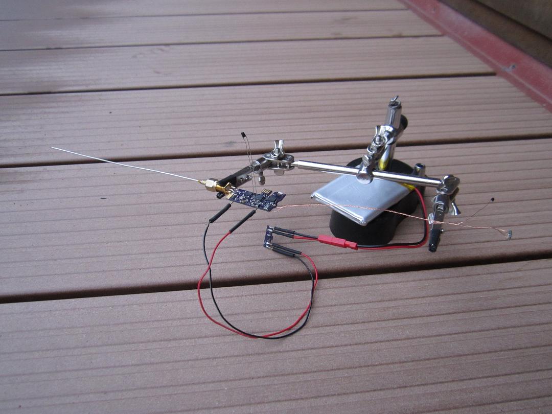
TX Antenna
Since long distance transmission wasn't necessary throughout development, just an unmatched short wire antenna was used for convenience. In flight, the tracker will utilize the following antenna.


| Material | ρ [nΩm] | μr | δ [μm] | Rc [Ω] | Eff. [%] |
|---|---|---|---|---|---|
| Copper | 16.8 | 1.0 | 5.4 | 2.7 | 93.1 |
| Brass | 70.0 | 1.0 | 11.1 | 4.1 | 89.8 |
| Carbon Steel | 143.0 | 100.0 | 1.6 | 38.9 | 48.1 |
| Stainless Steel | 690.0 | 1.0 | 34.7 | 11.2 | 76.2 |
Another variable that affects the antenna's performance is the material from which it is made. Since it is desirable the antenna weighs as little as possible, thin guitar strings have become popular source of antenna material on many trackers. A thin enameled magnet wire has also been frequently utilized particularly on HF frequencies. The guitar strings I've managed to get hold of are labeled as Bronze Wound .008p (0.2mm in diameter), High Carbon Steel (0.25mm) and Plain Steel .013p (0.33mm). The manufacturer doesn't share any more details on inner composition of the strings. Other sources suggest that underneath the winding there is typically a high carbon steel core in case of the wound strings. Although, there was no information on the thickness of the individual layers. The table above compares the antenna's performance when the driven element (0.2mm in diameter) is constructed from different materials. The two ground elements are in all cases modeled as copper wires 0.1mm in diameter to represent the magnet wire. The first column contains the material's resistivity $\rho$, the second relative magnetic permeability $\mu_{r}$, then the resulting skin depth $\delta$ at 145MHz, the conductor resistance $R_{c}$ of the whole antenna, and finally the resulting antenna efficiency assuming a 36Ω radiation resistance. The resistivity and permeability values in case of the steels should be taken only as an example, since in case of steel, there is a large variety of specific alloys with differing properties. It is apparent that the performance is deteriorated the most by materials with high magnetic permeability which is not a good news for the guitar strings I have, because all responded to a magnet when tested. On the other hand, both the Bronze Wound and Plain Steel guitar strings were verified to work sufficiently as antenna materials on my previous TT7F flights, or rather neither caused a noticeable reduction in transmission range at respective output powers. Similarly, the enameled copper magnet wire was proven to work as an antenna on TT7F6W which transmitted on both APRS and WSPR frequencies. Since the guitar strings were very thin (0.2mm) and the thickness of the bronze winding is unknown, it is unclear whether skin effect kept the currents in the low loss bronze layer, or the core material simply doesn't deteriorate the performance that much.


Final Performance Test
Once all the individual parts described in the previous paragraphs were finished, it was time to see how the tracker performed on its own.


Conclusion
At this point the tracker is firmware-wise and hardware-wise ready for a flight that would assess its performance in the actual environment it was intended for. All the necessary information to build a TT7B tracker including the firmware, PCB schematic and board design can be found in this blog post, the previous post and the Github repository.
Notes
While I was working on the firmware, I put together a second tracker as the soldering paste I had was approaching its expiration date.


Note: In the end, I desoldered the TPS3831 supply voltage monitor from the second tracker as well. The reason was that the relatively high threshold voltage (1.628V-1.695V) kept causing too many unnecessary external resets particularly at lower temperatures resulting in gaps in the backlog. A lower threshold model such as TPS3831E16 (1.482-1.543V) should be tested.
Hi, I saw your comment on habhub irc about soldering solar cells, the trick is to solder at a lower temperature, I set the temp to 330° instead of the 390 im usuly use when soldering, that way it does not destroy the solderpads on the cells and makes it 100 times easier to solder.
ReplyDelete73
/Mikael
Hi Mike,
DeleteI was soldering them at lower temperature as well in the end, but it still wasn't great. I tried all sorts of things: filing the surfaces, using different flux. But nothing lead to a 100% success rate. Maybe it's just in the hands :-).
Hi, You write about handling the case where battery drops bellow 0.75V due to cold but I didnt found any mention of reset circuitry for TPS610xxx converter which gets locked up under 0.7V too. Did I missed something or that wasnt a problem?
ReplyDeletebtw. you should be able to use any SWD programmer to program any ARM chip with SWD. You dont need to get special programmer just for a SAM chips. (You can use raspberry pi zero as universal ARM programmer too)
Hi,
Deletethe main TPS61099 doesn't have any reset circuitry. It simply stops outputing the programmed voltage when the input voltage falls below 0.7V. When the input voltage rises above 0.7V, or so, the converter starts outputting the desired voltage again. The tracker was designed with an MCU supervisor which in the end wasn't used. During an actual flight, the lowest reported battery voltages (Energizer Ultimate Lithium) were 1.2-1.3V. What was happening with the tracker/voltages during the periods the tracker didn't transmit, typically during night-time, is unknown.
At the time I was designing the tracker, the only cheap solution I came across to program ARM MCUs was ST-Link V2 from Ebay which could do only STM MCUs as far as I know. Any links to the RPi programmer?
Tomas
Asking because according to datasheet TPS610xx should get into lockout when it shutdsdowns and you need to do reset on EN pin or remove voltage completely.
DeleteThis is solid start point https://learn.adafruit.com/programming-microcontrollers-using-openocd-on-raspberry-pi/overview also another thing I tend to use is J-link clones from ebay which you can find when you search for "OB ARM Debugger" they work fine with J-link 5.00, never software has problems with them.
The datasheet I have - TPS61099 Revised May 2018 - doesn't mention requiring EN pin reset when the IC goes to lockout. The actual behavior of the tracker supports that. During testing, I fed it voltages from a bench PSU varying it across the whole range 0-1.8V in 10mV steps. It never had an issue starting up again when the input crossed roughly 0.7V.
DeleteThanks for the link, I'll look into that. The other reason I went with the solution I used was that I knew it supported debugging. Just had to make it work.
Tomas
I see now, thats only a issue with TPS6100x
Delete
ReplyDeleteVehicle Tracking Devices Jaycar
if are you buy the GPS Car tracking system then we provide the best GPS vehicle tracking system by Autos Ghana Limited, for Vehicle Tracking Devices, contact us.
to get more - http://www.autosghana.com/gps-tracking/gps-vehicle-tracker/
Online driving license tracking makes it easy to monitor your license application or renewal from anywhere. With real-time status updates and accurate information, drivers can avoid delays and unnecessary follow-ups. Using Online Driving License Tracking in the middle of your process ensures transparency, saves valuable time, and keeps you informed at every step. It’s a convenient, reliable way to stay updated and stress-free.
ReplyDelete