A year ago, I wrote a blog
post about transmitting small SSDV images over a relatively slow RTTY link. Already back then, I was aware of the limitations and that there were solutions with better image quality and higher transmission speeds. Particularly,
Dave Akerman's approach developed around small accessible LoRa modules raised my interest. I ordered a pair, a new camera, and started experimenting. This blog post now summarizes what I eventually came up with.
LoRa - Long Range
LoRa is a name for a patented modulation scheme present in Semtech's transceiver ICs and a variety of ready-made modules. Although, there have been successful attempts to demodulate and decode LoRa transmissions with a software defined radio and an extra module for GNU Radio, I am not aware of it being implemented into any of the widespread SDR applications so far. So the surest way of doing something with LoRa, for now, is having two modules.
In principle, all that needs to be done to establish a simple link is interconnecting the LoRa module with a microcontroller via an SPI interface, configuring the transmit frequency and specific modulation parameters, and then simply feeding the module packets of data. The IC does all the encoding and modulating on its own. On the receiving side, a microcontroller configures another LoRa module with the same parameters, switches it to RX Continuous mode, and either waits for an interrupt signalling a received packet, or repeatedly polls for RxDone flag which signals the same. In more complex scenarios, the receiving module can mostly sleep and receive only at certain times. Or the two modules can be time synchronized to allow two-way communication switching between receive and transmit modes of operation.
Parameters. The modulation parameters mentioned previously determine the signal's 'appearance' in the frequency spectrum and affect the transmission's potential range, its bit rate and interference resilience. They are spreading factor, modulation bandwidth and error coding rate. Spreading factor determines how many bits are encoded into each transmitted symbol (6 to 12). Higher values slow down the data rate and increase range. Bandwidth sets the amount of occupied spectrum by the modulation. It ranges from 7.8kHz to 500kHz with higher bandwidths increasing the data rate. And finally, error coding rate represents the amount of additional data sent with each packet to perform forward error correction at the receiver. The selectable data overhead ratio ranges from 1.25 (4/5) to 2.00 (4/8). In this case, larger the overhead, more corrupt bits the algorithm can correct. There is also an option to select between explicit and implicit header mode which decides whether the transmitted packet includes information about its length, its FEC rate, and whether it includes a CRC or not. Transmissions with spreading factor 6, for example, always require the use of implicit header mode.
| Mode |
Header |
BW [kHz] |
ECR |
SF |
BR [bps] |
| 0 |
explicit |
20.8 |
4/8 |
11 |
43 |
| 1 |
implicit |
20.8 |
4/5 |
6 |
1476 |
| 2 |
explicit |
62.5 |
4/8 |
8 |
915 |
| 3 |
explicit |
250.0 |
4/6 |
7 |
8509 |
| 4 |
implicit |
250.0 |
4/5 |
6 |
17738 |
| 5 |
explicit |
41.7 |
4/8 |
11 |
104 |
| 6 |
implicit |
41.7 |
4/5 |
6 |
2959 |
| 7 |
explicit |
20.8 |
4/5 |
7 |
841 |
| 8 |
implicit |
62.5 |
4/5 |
6 |
4435 |
| 9 |
implicit |
500.0 |
4/5 |
6 |
35476 |
Since there already was a widespread LoRa based system for high altitude ballooning in the form of Dave Akerman's PITS, I adopted the nine 'LoRa modes' already in use, so my transmitters would be compatible. I added Mode 9 on top of that for testing the highest data rate configuration LoRa provides. The table above summarizes the parameters of individual modes and provides a calculation of an effective bit rate. The equations can be found in the IC's datasheet, and the bit rate value is valid for a 255 byte packet (one SSDV packet for example). Since this is not actual bit rate, but a value derived from time on air of such packet divided by the size of only the payload data, the effective bit rate decreases with less data sent by the user. For example, when transmitting only a 50 byte packet (short UKHAS style telemetry string) in Mode 4 the effective bit rate decreases from 17738 to 14302 bps.
Modulation. To provide some visual aid, the above is a screen grab of a Mode 0 packet in SDRsharp's waterfall (horizontal axis represents frequency, vertical axis time). The signal is comprised of a series of up-chirps and down-chirps all within the selected bandwidth. Data is then represented by instantaneous changes in frequency between individual chirps. All of this including the whole demodulation and decoding process is brilliantly described in
this presentation by Matt Knight.
This is what a LoRa transmission looks like in SDRsharp's spectrum analyzer screen. Left to right: 20.8kHz, 41.7kHz, 62.5kHz and 250kHz bandwidth. The signal level decreases as the energy is spread across a wider bandwidth.
To better imagine the difference between individual modes, in other words the parameters, this is a screen grab from SDRsharp's waterfall again capturing the same 57 byte packet transmitted by all ten modes in succession with 250ms gaps in between transmissions. From the bottom up: the slowest Mode 0, then Mode 1, all the way to a very fast and quite faint Mode 9. Note the varying bandwidths and on air times.
Hardware. The modules I opted for were HopeRF's RFM96 intended for the 434MHz band, ordered on Ebay. Comparing Semtech's and HopeRF's datasheets, it seems that the modules simply use the Semtech's SX127x ICs while mainly providing the external filtering and impedance matching for a specific frequency band. I also designed simple adapter boards which now host my modules. At the time, I was experimenting with AX5243 transceivers as well, so there is its layout on the backside of the board. The output of the two transceivers is handled by a BGS12SN6 RF switch (LoRa being the default output). For anyone interested in a closer look:
AX5243.brd and
AX5243.sch.
Once I wrote some basic software, I went on to measure the power output of all three modules (I eventually ordered a third one) with
AD8313 that I had previously used on the same task with
Si4463. The datasheet describes two output options, namely PA_HP amplifier on PA_BOOST pin and PA_LF on RFO_LF pin each with different power range and step size. However, the modules output power only when PA_BOOST was selected which made me wonder whether the other output was connected on these module or not. I wasn't able to tell from simply looking at the boards.
Nevertheless, these are the measurements, and they suggest something very wrong with two out of the three modules. One module in terms of power and consumption behaved to expectation. In case of the remaining two, there has to be something wrong with their TX side, because as the following data suggest, in reception, the two outperformed the good transmitter.
| Mode |
RFM_TX |
RFM_ST |
RFM_HH |
Thermal |
| 0 |
-92.4 dBm |
-103.8 dBm |
-102.7 dBm |
-130.8 dBm |
| 1 |
-92.9 dBm |
-103.3 dBm |
-102.2 dBm |
-130.8 dBm |
| 2 |
-87.0 dBm |
-98.0 dBm |
-96.6 dBm |
-126.0 dBm |
| 3 |
-78.9 dBm |
-91.8 dBm |
-90.3 dBm |
-120.0 dBm |
| 4 |
-79.4 dBm |
-92.1 dBm |
-90.7 dBm |
-120.0 dBm |
| 5 |
-87.9 dBm |
-98.6 dBm |
-97.1 dBm |
-127.8 dBm |
| 6 |
-88.0 dBm |
-98.9 dBm |
-97.0 dBm |
-127.8 dBm |
| 7 |
-93.0 dBm |
-103.2 dBm |
-102.0 dBm |
-130.8 dBm |
| 8 |
-86.6 dBm |
-98.0 dBm |
-96.5 dBm |
-126.0 dBm |
| 9 |
-75.5 dBm |
-88.0 dBm |
-87.0 dBm |
-117.0 dBm |
Reading RegRssiValue register and performing necessary adjustments detailed in the datasheet provides the user with an RSSI (Received Signal Strength Indicator) value in dBm which represents the momentary power present in selected bandwidth at the frequency the receiver is tuned to. Similar power readings are available after each received packet in the form of the packet's RSSI and its signal to noise ratio (SNR). Initially, there was some confusion about what offset to use to get a legitimate reading. The Semtech's datasheet provides an offset of -164, but states that the value is dependent on the RF front-end (matching, filtering, etc.). The HopeRF's datasheet, though, provides a 27dB higher value of -137. I eventually fed a 2.9dBm output of RFM_TX directly to the receiving RFMs through a 30dB attenuator and had them measure the packet RSSIs. On average, after adjusting for the attenuation, the readings returned power levels of -3.2dBm and 0.6dBm while using the -137 offset and levels of -30.3dBm and -26.5dBm when -164 was used favouring the HopeRF's datasheet. The table above then contains averaged RSSI readings of all three modules connected to an antenna in different LoRa Modes. As no LoRa transmissions were made during that time, the readings represent the noise floor individual modules saw. For comparison, the last column contains computed thermal noise levels at 17°C (290K) for respective bandwidths. $$P = k_{B}TB$$where $P$ is the power in Watts, $T$ is the noise temperature in Kelvin, $B$ is the receiver bandwidth in Hertz, and $k_{B} = 1.381 \times 10^{-23}\;J/K$ is the Boltzmann constant. The thermal noise here represents the unavoidable noise generated within a receiver itself by moving charge carriers due to its temperature. As the bandwidth increases the amount of noise power increases as well. It is apparent that the modules are quite noisy with the 'good transmitter' being further 10-11dB noisier than the other two. Coincidentally, RFM_TX is the only board that has the AX5243 on the other side populated, and even though it was powered off, I can't rule out the possibility it was somehow responsible for the increased noise.
| F [mHz] |
F [mHz] |
P [mW] |
BW [kHz] |
DC [%] |
Area |
| 433.05 |
434.79 |
10 |
|
10 |
CZ, UK |
| 433.05 |
434.79 |
1 |
|
|
CZ, UK |
| 433.05 |
434.79 |
10 |
25 |
|
CZ |
| 434.04 |
434.79 |
10 |
25 |
|
UK |
Frequency Bands. Reading through documentation, there are slight differences between the UK and the Czech Republic which is where I am. In case of Britain, I drew from Ofcom's IR2030 that is aimed at licence exempt short range devices. For the Czech Republic, the information is contained in VO-R/10/12.2017-10 in section on short range devices. There are three options in either country. The first limits transmissions in power to maximum 10mW e.r.p. (effective radiated power) which means the power output by the transmitter plus the antenna gain over dipole in its main lobe (dBd = 2.15dBi) mustn't exceed 10mW. And it also adds a maximum duty cycle limit of 10%. The second option doesn't restrict the bandwidth nor the duty cycle, but strangles the power to only 1mW e.r.p. And finally, the third option, which differs in the frequency range between the two countries, limits the power to 10mW e.r.p. and the bandwidth to 25kHz.
Link Budget. Taking all the information from above, it is possible to make some basic link budget estimates. The picture illustrates the situation. There is a transmitter on a balloon with an antenna, a receiver on the ground with another antenna, and there is a line of sight in between the two. A radio horizon given by the curvature of the Earth for a balloon at a certain altitude can be approximated with the following equation: $$d = \sqrt {2 \cdot k \cdot R \cdot h}$$ where $d$ is the distance in meters, $R$ is the Earth's radius in meters, $h$ is the balloon's altitude in meters, and $k$ is a factor which takes into account the refractive effects of the atmosphere (k = 4/3 during normal weather conditions) on the propagating signal. The radio horizons for balloons at 10km and 30km in altitude, for example, are 412km and 714km respectively.
| Mode |
SF |
S/N |
RFM_ST |
RFM_HH |
| 0 |
11 |
-17.5 dB |
-121.3 dBm |
-120.2 dBm |
| 1 |
6 |
-5.0 dB |
-108.3 dBm |
-107.2 dBm |
| 2 |
8 |
-10.0 dB |
-108.0 dBm |
-106.6 dBm |
| 3 |
7 |
-7.5 dB |
-99.3 dBm |
-97.8 dBm |
| 4 |
6 |
-5.0 dB |
-97.1 dBm |
-95.7 dBm |
| 5 |
11 |
-17.5 dB |
-116.1 dBm |
-114.6 dBm |
| 6 |
6 |
-5.0 dB |
-103.9 dBm |
-102.0 dBm |
| 7 |
7 |
-7.5 dB |
-110.7 dBm |
-109.5 dBm |
| 8 |
6 |
-5.0 dB |
-103.0 dBm |
-101.5 dBm |
| 9 |
6 |
-5.0 dB |
-93.0 dBm |
-92.0 dBm |
The datasheets state that depending on the transmission's chosen spreading factor the receivers should be able to successfully decode signals down to different levels below the noise floor. Higher the spreading factor, lower the signal level can be. The table contains these values for respective LoRa Modes. The last two columns then consist of the previously measured levels of noise floor adjusted for this value in case of the two better receivers. This figure then represents the lowest signal level in absolute terms the specific receiver should be able to decode.


The diagrams above illustrate the radiation patterns of two possible receiving antennas. The top left is the pattern of a ground plane antenna placed 8.5m above real ground (my roof top) as modelled by 4nec2. The remaining three represent a 7 element Yagi antenna again 8.5m above real ground at three different elevation angles (0°, 45° and 90°). A closer look at the gain distribution of the ground plane antenna as elevation of a hypothetical balloon increases reveals that from a maximum of 3.6dBi at 12.5° the gain decreases to -3dBi at a 45° angle till it drops completely when the balloon gets directly overhead. The gain of the Yagi antenna then is only as good as one's ability to direct it towards the balloon. Similarly to the receiver, an antenna produces noise which in its case depends on its environment and radiation pattern. As I am given to understand, unless a high gain antenna is directed at the Sun (strong source of radiation), its contribution to the overall system's noise can be neglected. The last element to complete the receiving chain is the transmission line between the antenna and the receiver. For an example, I will use 5m of a coaxial cable adding 3.15dB in feeder loss. $$FSPL = \left( \frac{4 \pi d}{\lambda} \right) ^2$$ Free-Space Path Loss represents the decrease in power density proportional to the square of the distance $d$ the signal has travelled from the transmitting antenna to the receiving antenna. The equation assumes isotropic antennas (0 dBi) for the specific wavelength $\lambda$. In other words, power is received through a smaller area (antenna aperture) in case of shorter wavelengths than it is in case of longer wavelengths (larger antenna aperture). Hence the seeming dependence of power density decrease on wavelength. Aside from the free-space path loss, total path loss may take into account additional losses specific to the environment in which the signal propagates if such losses are known.
Equivalent Isotropic Radiated Power (EIRP) represents the power that would have to be radiated by an isotropic antenna to give the same power density as the transmitting antenna in a specific direction. It is used to quantify the initial amount of power leaving the transmitter in a direction of the receiver for the link budget calculation. A related concept, Equivalent Radiated Power (ERP), was introduced in the section on frequency bands and legal limits. The difference between the two is in the antenna used as the reference which is a half-wave dipole in case of ERP and a theoretical isotropic antenna in case of EIRP. The EIRP value is 2.15dB larger than ERP. In a situation where there is a legal limit on transmitted power, the sum of the transmitter's output power and of the gain of the antenna in its main lobe has to fit within this limit.


Probably the most often used transmitting antenna on high altitude balloons is an inverted ground plane antenna. The difference to its usage near actual ground is that the radiation pattern and hence its gain is very similar to a half-wave dipole's pattern. Both modelled in free space by 4nec2 in the diagrams above (ground plane left, half-wave dipole right). The four radials can't replace real ground. Their advantage lies in simplifying impedance matching as opposed to matching the dipole. All that needs to be done is bending the radials at an angle (about 45°) away from the radiating element to match the antenna to a 50
Ω coaxial cable. The maximum gain of both antennas was modelled to about 2.1 dBi, and to -1.17 dBi in case of the ground plane and -1.88 dBi in case of the dipole when evaluated at a 45° angle. $$FSPL_{max} = EIRP_{(dBm)} - RX{\_}Min_{(dBm)} + RX{\_}Ant_{(dBi)} - Feeder_{(dB)}$$ Now, to start putting it all together, the equation above expresses the maximum free-space path loss $FSPL_{max}$ in dBm for specific choice of parameters, so the transmitted signal is still decodable. The receiving antenna gain $RX{\_}Ant$ is added, the minimum signal level $RX{\_}Min$ and feeder losses $Feeder$ are subtracted from the $EIRP$ value. Note that all values are expressed in their decibel form. $$d_{LOS} = \frac{\lambda \sqrt{FSPL_{max}}}{4 \pi}$$ This equation then calculates the line of sight distance $d_{LOS}$ in meters which corresponds to the free-space path loss $FSPL_{max}$ at wavelength $\lambda$. Since this whole post deals with 434MHz LoRa modules, the wavelength used in the following table is 0.691m. Also note that the $FSPL_{max}$ value was converted to mW form for this calculation.
| Mode |
Tx Pwr |
Tx Ant |
Tx EIRP |
Rx Ant |
Feeder |
Rx Min |
LOS |
Info |
| 0 |
10 mW |
2.1 dBi |
16.2 mW |
3.6 dBi |
3.15 dB |
-121.3 dBm |
271.0 km |
~34bps |
| 0 |
10 mW |
-6.0 dBi |
2.5 mW |
-6.0 dBi |
3.15 dB |
-121.3 dBm |
35.3 km |
~34bps |
| 1 |
10 mW |
2.1 dBi |
16.2 mW |
3.6 dBi |
3.15 dB |
-108.3 dBm |
60.7 km |
1.5kbps |
| 1 |
10 mW |
2.1 dBi |
16.2 mW |
11.4 dBi |
3.15 dB |
-108.3 dBm |
148.9 km |
1.5kbps |
| 4 |
1 mW |
2.1 dBi |
1.6 mW |
10.5 dBi |
3.15 dB |
-97.1 dBm |
11.7 km |
17.7kbps |
This table summarizes a few scenarios in which a high altitude balloon and a receiving station might happen to be and provides values for the maximum line of sight distance in kilometers at which the signal from the balloon should be decodable. The first row, for example, assumes a distant balloon transmitting a telemetry string in LoRa Mode 0 (20.8kHz, ~50 byte packet at 34bps). These parameters allow transmitting 10mW ERP which corresponds to setting the transmitter to output 10mW into a ground plane antenna (the EIRP value is then 16.2mW). Since a balloon at a distance is assumed, the low elevation gain of 3.6dBi can be used for the receiving ground plane antenna. The lowest power level in this mode my LoRa module should be able to decode is -121.3dBm. That results in 271km maximum line of sight distance for this link. The second row, on the other hand, assumes the same balloon to be almost above the receiving station which requires assuming much lower antenna gains (see the radiation patterns) and results in much shorter range. The next two rows in the table compare the ranges of higher data rate LoRa Mode 1 (20.8kHz, 255 byte packet at 1.5kbps), often used for SSDV, when received with a ground plane antenna and a Yagi. The last row then shows that the wide band (250kHz) very high data rate (255 byte packet at 17.7kbps) LoRa Mode 4 is limited to only 1mW ERP (1.6mW EIRP) and would have a very short range even with a receiving Yagi antenna.
Looking at the link as a whole, the obvious weakest link are the very noisy LoRa receiver modules. It may be worth it to order a couple of modules from other manufacturers and compare them. Also note that these are all theoretical computations and assumptions yet to be confronted with reality. Nevertheless, these previous paragraphs give an idea of what could be done on air given the tools as described. Now, lets look at the actual content that may be transferred via these links.
Update. After finishing the previous paragraphs, I ordered a couple more modules and some accessories to do further testing. Both the modules were SX1278 based and among the cheapest found on Ebay. Since I didn't have any adapter boards for these, I had to solder the SMA connectors and pin connections directly as in the photos above.

First, I repeated the TX power measurement with AD8313 for all five modules. The two new SX1278s performed comparably to the 'good' RFM96 transmitter, both in TX power and current consumption. The shielded module is denoted as SX1278_SH while the other one as SX1278_BL (blue). $$RSSI [dBm] = -137 + RegRssiValue$$ The ICs in all the modules provide three registers, as mentioned previously, that contain measurements of RSSI, packet SNR and packet RSSI. The above and the following equations then illustrate how to convert the register readings to the actual values. They are also used in the code I wrote. $$SNR [dB] = \frac{RegPktSnrValue}{4}$$ The SNR reading is useful in situations where the signal level is below the noise floor. According to discussions on Semtech's forum, reported SNR values above +5 are inaccurate and can be interpreted as simply 'enough signal'. This is reflected in my code by using this threshold to report the SNR either according to the equation above or as the RSSI value representing the current noise floor subtracted from the packet RSSI value. $$PacketRSSI [dBm] = -137 + 16/15 \cdot RegPktRssiValue$$ The datasheet proposes adjusting the register reading by 16/15 in cases the SNR is positive to compensate for the non-linearity of the packet RSSI measurement. $$PacketRSSI [dBm] = -137 + RegPktRssiValue + \frac{RegPktSnrValue}{4}$$ In case of packet receptions below the noise floor, the SNR value is subtracted from the packet RSSI reading. Both RSSI and packet RSSI computations include a fixed offset of -137. This value comes from the HopeRF's datasheet. I couldn't find this offset for either of the new SX1278 modules, so -137 was used with them as well.
| Mode |
RFM_TX |
RFM_ST |
RFM_HH |
SX_BL |
SX_SH |
| 0 |
-102.0 |
-104.1 |
-102.4 |
-92.8 |
-101.6 |
| 1 |
-102.4 |
-104.5 |
-102.4 |
-93.5 |
-101.5 |
| 2 |
-97.2 |
-98.8 |
-97.5 |
-88.4 |
-95.8 |
| 3 |
-90.8 |
-93.4 |
-90.8 |
-82.1 |
-90.1 |
| 4 |
-90.7 |
-92.5 |
-91.2 |
-80.8 |
-89.0 |
| 5 |
-97.9 |
-99.6 |
-97.9 |
-88.8 |
-95.7 |
| 6 |
-97.1 |
-99.5 |
-98.0 |
-88.3 |
-95.9 |
| 7 |
-102.2 |
-104.7 |
-102.2 |
-93.6 |
-100.7 |
| 8 |
-96.7 |
-99.0 |
-97.1 |
-87.9 |
-95.7 |
| 9 |
-87.3 |
-90.2 |
-88.1 |
-77.8 |
-87.0 |
This is a summary of averaged RSSI measurements of all five modules in all individual LoRa modes for when there were no LoRa transmission on air. I have noticed some of the modules being quite sensitive to slight variations in the overall setup, so in putting this table together, I tried maintaining the same conditions. The modules were connected to a 70cm ground plane antenna via a 2m coaxial cable and Arduino ProMini with a USB to UART bridge. The idle RSSI readings were sent to a PC every second for a couple of minutes in each mode. The modules were swapped in succession. Contrary to the original test the RFM_TX performed comparably to the other two RFM96s. The shielded SX1278's noise floor seemed to be similar or slightly worse. In case of the blue SX1278, the RSSI readings were about 10dB worse across the modes. I did all of this twice, first with the modules as they were, then inside an aluminium box. The results were very similar in both cases.


To establish whether the difference in SX1278_BL's noise floor was due to the offset value being different for this module, and to evaluate the accuracy of the -137 offset in the other modules, I thought I would test this with a few attenuators. I bought these four 30dB SMA pieces, and while I was waiting for the delivery, I built another homemade 20dB attenuator following
this W2AEW's video.
The idea was to use one of the modules with a known output power to transmit directly to the individual receivers through these attenuators, and confront the reported packet RSSI and SNR values with expected levels based on the attenuation used. I did all sorts of variations of these measurements: the TX and RX modules connected only by the attenuators, at a distance separated by a coaxial cable, attenuators placed closer to the transmitter, then to the receiver, different levels of attenuation, shielding the transmitter, and so on. In the end, it became obvious that the setups were leaking RF somewhere corrupting the measurements. Further reading on this topic suggests that these sorts of tests require much more care in avoiding RF leakage. Using double shielded coaxial cables was mentioned, for example, in achieving these high levels of attenuation.
As a result of these efforts, I became somewhat uncertain about the reliability and accuracy of the reported RSSI, packet RSSI and SNR values by these modules in absolute terms. This could influence the previous results of the link budget calculations, but at least the general principles should stand.
OV5640 Camera Module
Seeing images from the PiCamera, which is equipped with OV5647 sensor, regularly on the SSDV page, and finding all sorts of similar models available on both Ebay and Aliexpress, I thought that it would be a good step forward from the MT9D111 I had used previously.
The first sensor I ordered was this OV5640 with a wide angle lens and a 24 pin flex cable. There are a few similar versions that pop up in the search engine, but differ in pinout.
One other that is more or less compatible was this narrow lens OV5640 sensor equipped with autofocus which I bought later on as well. The slight difference was that one of the NC (no connection) pins on the previous sensor was used as autofocus ground (AF-GND) on this one.
Since I already had some idea on what it takes to make things work with these sorts of modules, I designed this adapter board to make it easier for myself. All the useful pins are accessible in a 2.54mm pitch, there are two regulators to provide the necessary power supplies (1.5V and 2.8V from a 3.3V input), a pair of pull-up resistors for the I
2C lines, and it is equipped with an AL422B FIFO buffer which can hold up to 393,216 bytes of image data.

The idea was that unlike in my TT7F where I sampled the camera output directly and was limited by the size of the main MCU's RAM, I could use a simple Arduino to operate the camera and the buffer, and then extract an image from the buffer in small parts and at low speeds to process it. The schematic above illustrates the necessary connections to achieve this. Most of the AL422B's control pins are active low. One bit that may need explaining is the use of a NAND gate (SN74LVC1G00) between the HREF signal and the buffer's write enable (/WE) pin. The camera outputs a VSYNC signal indicating an active frame, HREF signal indicating an active image row (in case of JPEG this simply indicates valid data is present on the D7-D0 output lines), and PCLK signal clocking out the individual image bytes. The NAND gate then allows one to use only the transitions in the VSYNC signal to capture the whole frame in the buffer while taking care of the idle periods in the HREF signal automatically. After capturing an image, the Arduino can provide the buffer with a slow clock signal on the RCK line and sample individual image bytes on the DO7-DO0 pins. Note that the design also contains a footprint for a TCXO which, however, was not used in the end. The camera requires an external clock signal which I hoped to provide with the oscillator (I had a bunch of cheap TCXOs I wanted to test), but the amplitude of the output signal wasn't sufficient. Expecting a potential issue, the XCLK line was brought out among the 2.54mm pitched pins, so the TCXO can be omitted and the clock signal provided externally via the pin. As the note in the schematic suggests, for the autofocus sensor, I had to subsequently connect the outermost pin (NC2 -> AF-GND) to ground. I did that by scratching through the soldermask covering the main ground plane and connecting the two. I should also mention that I designed the board based on the main OV5640 datasheet and a schematic of a similar adapter which neither provided an excess of information. Only fairly recently, I came across an OV5640 application note that went in a little more detail about different power supply options and other hardware connections in general. This additional information suggests that my solution is not ideal and could be improved upon. For anyone interested, the original Eagle files can be downloaded from
here and
here.
Initially, I naively thought that I could solder the flex cable straight to the board, but it turned out to be a bit thicker than the cables I saw being soldered. Luckily, a suitable connector was easy to obtain from a local electronics parts wholesaler (that was much more problematic in case of the MT9D111 earlier). At first, I started to develop the camera software with Arduino Due, because it provided much more RAM and many more pins to connect the adapter to. After I succeeded and learnt more about which pins I needed and which I could do without, I moved to my original target which was Arduino ProMini. It turned out that with a couple of compromises the ATmega328p based board has just enough pins to make it work (taking into account SPI and UART pins reserved for communication to LoRa and GPS modules to make a complete tracker).

One of the necessities was to provide the XCLK signal to the camera by some other means. Arduino Due could generate fast enough signal on its own, but that was not going to work with a ProMini running at 8MHz and having no pins to spare. Luckily, I came across
this video where the author takes a look at LTC1799 oscillator which based on voltage it sees at its SET pin can produce a square wave signal from 1kHz to 33MHz.
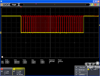
These are screenshots from Owon VDS1022I USB oscilloscope showing the LTC1799's output when set to 1MHz by a 50k
Ω potentiometer for illustration, and then the final choice of frequency actually used to run the camera (20MHz). In the latter case, the shape of the signal is not reproduced precisely as the oscilloscope's bandwidth is only 100MHz resulting in just 5 samples per wavelength.
The next step was establishing communication over the SDA (yellow) and SCL (red) lines between the Arduino and the camera's MCU. The above is an example of reading Chip ID registers (0x300A and 0x300B) via the I
2C interface.
The camera is then fed a long initialization sequence which sets up the internal PLL and all sorts of clock signals including the output PCLK. It adjusts the frame parameters, enables JPEG compression, and also writes a number of undocumented registers before it eventually enables the output (VSYNC, HREF, PCLK and the D7-D0 pins are by default disabled). The documentation provides example init sequences for different desired outputs, but unfortunately it isn't very open on general principles of the camera's operation, so too much tinkering with the registers usually ends with no output at all. I found it best to use already proven register settings and implemented the
ArduCam sequences with small adjustments. The above is an example of the activity on VSYNC (red) and HREF (yellow) lines after the initialization sequence. Each frame is fixed length (420ms) while the liveliness of the HREF line is determined by image resolution and quality - the amount of data to be transferred in each image.
This is a closer look at VSYNC and HREF again around the end of an old and the beginning of a new frame. To maintain a specific frame rate, the frame length is fixed (420ms) with the first data appearing about 150ms after VSYNC goes high leaving enough time for the ATmega328p to react to the transition and enable writing to the buffer.
This is a detailed look at HREF (yellow) and the pixel clock PCLK (red) which is fed to the AL422B's WCK pin (write clock). The buffer can operate with up to 50MHz input clock. With this specific initialization sequence and 20MHz input clock, the PCLK runs at 11.7MHz.
The Arduino ProMini has two read only pins in A6 and A7. One of these (ADC6, as denoted in the ATmega's datasheet) is used to sample the VSYNC line (red) for beginnings and endings of frames. When AL_capture_frame() function is called, it identifies the beginning of the frame and enables writing to the buffer by pulling the adapter's pin WE (yellow) high. It then continues to sample VSYNC until the end of the frame at which point it pulls WE low.
This is a closer look at how fast the function reacts to the VSYNC (red) transitions. In this case, WE (yellow) went high 100us after VSYNC and was pulled low 50us after the frame ended. I should also mention that VSYNC is in this ProMini implementation wired straight to the buffer's /WRST pin, so every high to low transition automatically reinitializes the buffer's write address to 0x00.


Reading the buffer begins with resetting the read address (pulling /RRST pin low) alongside manually emulating read clock by pulling RCK pin (red) low and high in turns. The individual instructions are padded with a 1us delay. After the reset sequence, reading is enabled by pulling /RE pin (yellow) low after which data is output at the DO7-DO0 pins at each rising edge of RCK. The 8MHz Arduino ProMini hits its potential, and as can be seen on the oscilloscope, the individual clock states get stretched. The screen grab on the left captures an SSDV buffer being filled with bytes of data while the screen grab on the right documents a much more instruction intensive checking whether the data in the AL422B contain a JPEG image. It also shows the read reset sequence right before /RE is pulled low. There is one more pin (/OE) on the AL422B that needs to be pulled low to enable output. As free pins on the Arduino are scarce, it is hardwired to ground in this implementation.


These screens once again illustrate the read process, this time on RCK (red) and D7 (yellow) lines. From the perspective of the Arduino the D7-D0 pins were connected in such a way that the image data byte is the result of ORed reads of PINB & 0b00000011 and PIND & 0b11111100 registers.
Getting the image is half of the job. The other half is processing it with the SSDV routines which in Arduino ProMini's case gets a little more complicated. Unlike the more powerful Arduino Due, ProMini is equipped with only 2048 bytes of internal RAM. At the heart of SSDV is a structure data type ssdv_t which contains a large number of variables and arrays that are used in the process. In the AVR environment, a variable called __brkval can be used to get the address of the top of the heap (which grows upwards inside the RAM) while the current position of the stack (which expands from the end of the RAM downwards) can be acquired as the address of the latest declared variable. With the help of these, one can get an idea of how much free RAM there is at different stages of code execution. In case of SSDV the heap stays the same throughout the whole code, but the stack expands by slightly over 1200 bytes. This is a large portion of the total and therefore care must be taken with the remaining processes.
/* Standard Huffman tables */
PROGMEM static const uint8_t const std_dht00[29] = {
0x00,0x00,0x01,0x05,0x01,0x01,0x01,0x01,0x01,0x01,0x00,0x00,0x00,0x00,0x00,0x00,
0x00,0x00,0x01,0x02,0x03,0x04,0x05,0x06,0x07,0x08,0x09,0x0A,0x0B,
};
The first necessary thing to do is storing all unchanging arrays in the MCU's flash memory. Otherwise they reside in RAM. This is achieved by declaring them with 'const' and 'PROGMEM' keywords as in the example above. This concerns all the ssdv arrays in ssdv.c, GPS UBX commands, and OV5640 register settings.
#include <avr/pgmspace.h>

// load_standard_dqt()
temp = pgm_read_byte(&table[i+1]);

// dtblcpy()
r = memcpy_P(&s->dtbls[s->dtbl_len], src, n);
Once stored in the flash memory the arrays have to be accessed with functions from the pgmspace.h library. That means all the ssdv functions using them have to be modified. An example of such modification is in the code snippet above. Another means of saving RAM is using one buffer for different purposes. For example in my code, LORA_pkt[256] is used to store the LoRa packet intended for transmission, it is used as the output buffer for SSDV routines at another time, and as a buffer for incoming UBX messages as well. It is also worth it to have a look at external libraries that are included in the project. For example, if the Arduino Serial library is used, it contains two 64 byte buffers which can be shrunk by redefining their size in HardwareSerial.h. Similarly, including the Wire.h library consumes 153 bytes of RAM. Therefore I made a simpler implementation of the I
2C interface which doesn't use any buffers. In the end, my complete tracker code that includes SSDV, GPS and LoRa routines when compiled takes up 436 bytes of RAM in global variables. The SSDV process adds about 1240 bytes when running. That leaves a room of 372 bytes for the stack to grow.
These then are a few example images taken by the two cameras, transmitted and received. The images on the left are from the wide angle lens module while the images on the right show the same scenery taken by the narrow angle lens. They are all 1024x768 pixels and encoded with SSDV quality 5 (70.8 JPEG quality).
The code running the tracker contains init sequences for nine different resolutions. These are an example of three of them taken by the wide angle lens and encoded with SSDV quality 6 (86.0). The first is 640x480 (30.4kB), the second 1024x768 (62.6kB), and the last 1280x960 (85.8kB).


In the process of acquiring an image in this way, there are two stages of JPEG encoding with their own quality settings. First is the camera's setting. Then the SSDV process re-encodes the image again before transmitting it. The three images above give an idea of different combinations of the two. The first image (26.0kB) was taken with the camera quality set to 50 and re-encoded with SSDV quality 4 (49.6). The second (32.3kB) with camera quality 93.7 and SSDV quality 4 (49.6). And the third (55.5kB) with camera quality 93.7 and SSDV quality 6 (86.0). The resolution of all three is 1024x768 pixels. It is apparent from the images that it is better to take a high quality image with the camera and then have the SSDV process limit its size.


In JPEG compression, the actual content of the image has a significant impact on the file size. These two 1024x768 pixel images were both taken with the narrow angle lens at camera quality 93.7 and SSDV quality 5 (70.8). However, the size of the first image is 63.3kB while the second grew to 186.6kB. In this application, larger JPEGs result in longer transmission times. For example, using LoRa mode 4, a 54.9kB image took 52s to transmit while 186.6kB one occupied the band for 2 minutes and 55s. It is therefore necessary to take all these variables into account when choosing image and transmission settings, and scheduling the frequency of telemetry strings among the image packets.


As mentioned previously, the second camera module is equipped with autofocus. This feature, however, requires downloading firmware, as it is referred to in the documentation, which in other words means writing more than 3 thousand undocumented registers to the camera. Once again, I had to find the actual firmware in other publicly shared
projects. After the firmware is stored in the Arduino's flash memory, the autofocus sequence works like this: write the firmware to the camera (based on my testing it has to be done before each focusing attempt), issue a 'single trigger' command by writing 0x03 to register 0x3022, keep polling register 0x3029 until it reads 0x10 signalling the focusing is done, issue command 'pause autofocus' by writing 0x06 to register 0x3022, capture the image, and finally release the lens by sending 0x08 to register 0x3022. The images above illustrate the results. For some reason, the focusing sequence takes about 10s which makes it highly impractical. Fixing the focus to infinity makes more sense on a balloon tracker anyway.


I also shouldn't pretend that everything works beautifully and mention a large number of erroneous images both cameras produce. As the above images illustrate, the errors range from MCU corruptions at a single spot which then propagate throughout the rest of the image, to multiple corruptions per image. I tried implementing an SSDV check of the captured image which if failed a new image would have been captured instead. However, even that managed to avoid transmitting only a portion of the corrupt images, and it also added substantial delays between individual image transmissions. Since the files when examined with JPEGsnoop don't show any errors, I am led to believe the source of the corruption is in the cameras themselves, not the subsequent buffer samplings and processing. Maybe a redesign of the power supply as mentioned previously could improve upon the error rate.
LoRa PAYLOAD
ProMini_LoRa_Payload.ino
OV5640_regs.h
ssdv.h,
ssdv.c,
rs8.h,
rs8.c
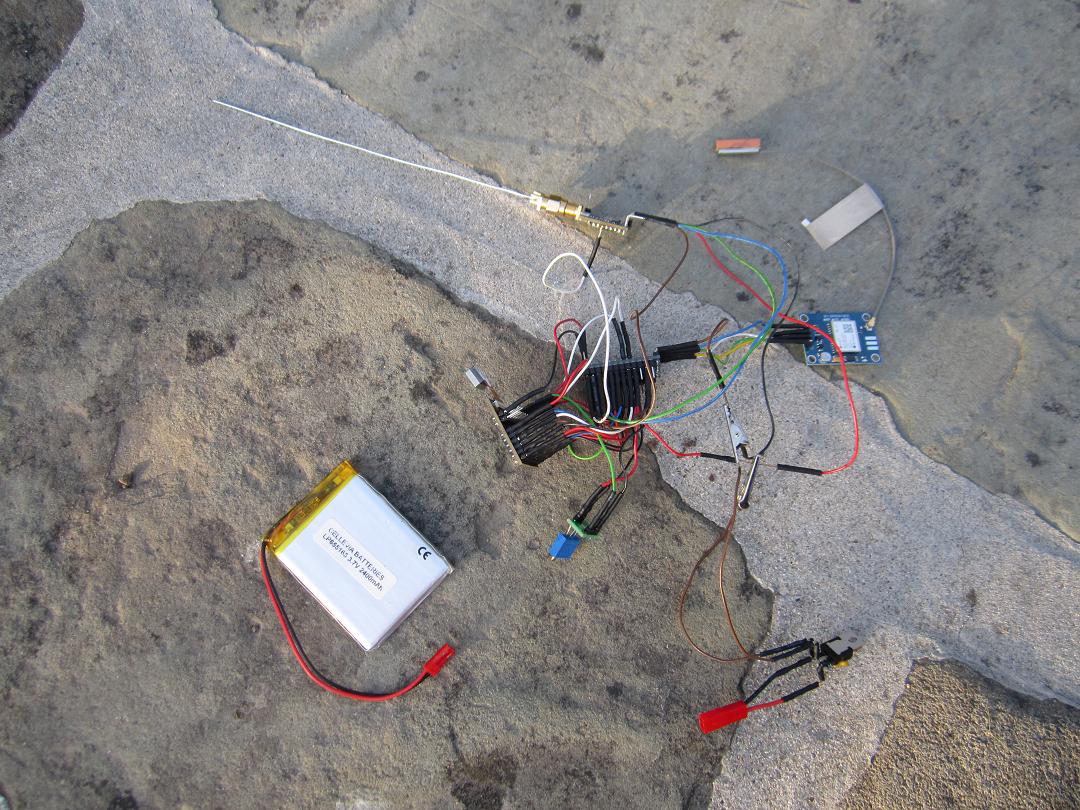
The two technologies discussed in the previous paragraphs eventually made its way into three pieces of hardware that together can establish a telemetry and ssdv link with optional upload of the received data to Habitat and SSDV servers. The first part is a high altitude balloon tracker.
A u-blox NEO-7M GPS module and an RFM96W LoRa transceiver were added to the parts already mentioned in the OV5640 section. The power supply was provided by a 3.3V external regulator LF33CV, here in combination with a LiPo battery which would be replaced by Energizer Ultimate Lithium cells for an actual flight. Likewise, a few pieces of polystyrene would make this still in development prototype a bit more secure.

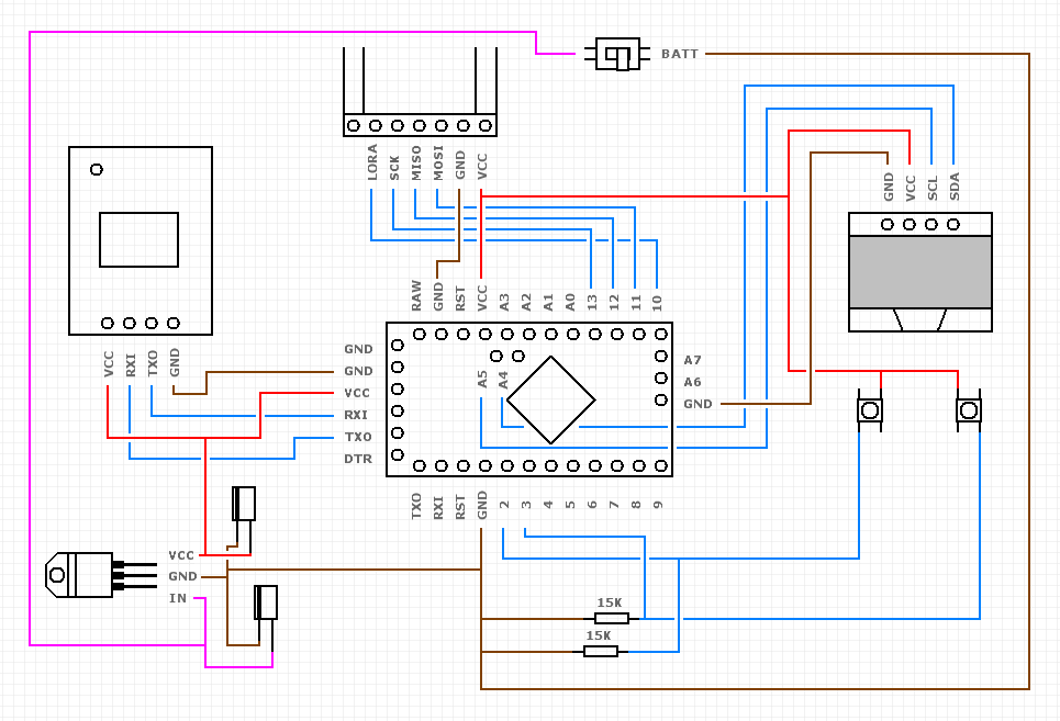
The complete wiring as hinted at in the previous paragraphs is shown in the schematic above. As can be seen, all controllable pins of the Arduino ProMini but one are used. The one remaining pin is read-only ADC7. The schematic also reveals that even though the datasheet suggests hard resetting the camera on power up, the ProMini doesn't have any spare pins to control the RST pin. Similarly, this implementation doesn't support powering the camera on and off via the PWR pin which is hardwired to ground. As I learnt from the late discovered application note, the power supply solution I had used on the adapter board also precludes from using the software power down option. Hence the camera runs continuously.

These oscilloscope screen grabs put some light on how long the SSDV processes take in the 8MHz ATmega328p. The image on the left shows the activity on RCK (red) and /RE (yellow) pins when the SSDV routine asks for more image data. A 32 byte IMG_buff[] is filled with data from AL422B and passed to SSDV. The image on the right shows the same from a higher perspective. Each SSDV packet required 11-12 data requests to complete with 12ms of processing time in between individual requests. That totalled to about 130ms to prepare a packet and another 130ms to transmit it with LoRa mode 4. This brings the effective bit rate of Mode 4 down to 8.2-8.5kbps (received image size divided by duration from the first image packet to the last).


I tried limiting the number of corrupt images in the final script by including an SSDV check in which every captured image is processed by SSDV, and transmitted only when the check succeeds. If it doesn't a new image is captured. The problem is that the time to process the image can take from 30 seconds to more than a minute per check (depending on image size). This adds delays in between image transmissions, and what is worse, it isn't able to catch all corrupt images anyway. So the usage of SSDV check is optional and decided by commenting or uncommenting SSDV_CHECK #define directive in the final script. In an afternoon of testing, the percentage of corrupt images without the SSDV check reached 28% (18/64) while the following set of images taken with the SSDV check exhibited 7.7% error rate (3/39).
The final script, provided at the beginning of this section, initializes the camera, the GPS and LoRa modules, and then enters the main loop. At the beginning of the loop a telemetry packet is transmitted. Following that an optional autofocusing routine is run if the AUTOFOCUS #define directive is uncommented. An image is captured and the AL422B is checked for its presence. An optional SSDV check is run, and in case of success, the main SSDV encoding and image transmission is initiated. In case of a failure, the scripts waits for 5 seconds and starts from the top of the main loop again. Both SSDV check and the main image transmission contain interleaved telemetry transmissions every X packets (configurable). Aside from that, the script includes an option to transmit a second slower telemetry packet on another frequency and a different LoRa mode right after the main transmission. This may provide distant listeners with telemetry reports in case the main transmission is in a high data rate mode such as 4 where its range is limited. The default settings for the final script are LoRa mode 4 on 434.250MHz at the lowest power setting (2dBm). The camera taking 1024x768 images in 81 JPEG quality transmitted in SSDV quality 50. I was looking for images in the range of 50-150kB. The optional slower telemetry is in LoRa mode 7 on 434.400MHz at 10dBm output power. SSDV check is turned on, autofocus off. All this can be easily modified in #define directives at the beginning of the script.
The SSDV and Reed-Solomon libraries at the start of this section are the RAM optimised versions that allow running SSDV on an Arduino ProMini. The original libraries can be found on Philip Heron's
Github.
Following up on the previous blog post about
GPS drift, the camera seems to interfere a little with the GPS receiver and increases the spread of reported positions by a stationary tracker. These maps come from two tests where the tracker was moved to capture different sceneries. The white dots represent the actual positions of the tracker, the blue then the reported ones.
These two charts show the payload's current consumption in different 10 second periods. First during SSDV check with a several hundred millisecond spike as the main and the slow telemetry packets were transmitted. Then at the beginning of image transmissions. In both cases the GPS was already running the less current consuming tracking engine. The average current consumption of the tracker was 130mA. The LiPo battery was charged to 3.91V at the time. The measurement was done as described later in this blog.
LoRa HANDHELD
ProMini_LoRa_Handheld.ino
fonts.h
The second piece of hardware that I put together is a battery powered handheld telemetry only receiver that displays the tracker's position, its own position, and calculates the distance, azimuth and elevation towards the tracker.
It's built from cheap Ebay parts which can be replaced and the whole thing taken apart. Once again it's run by an Arduino ProMini that gets its own position from a u-blox NEO-6 GPS module (the one that was part of my very first high altitude balloon). An RFM96W LoRa module then listens for transmissions from a tracker, and in case of a successful decode, the information is shown on a 128x64 pixel OLED display.
The wiring is illustrated in this diagram. I had to use an external LDO, because although the overall consumption was supposed to be within the capabilities of the Arduino's on-board regulator, the u-blox module seemed to be quite sensitive to clean power supply and refused to operate when the OLED was part of the circuit. An LF33CV 3.3V regulator with datasheet stated current output of up to 500mA solved the problem. The individual parts use all three interfaces of the Arduino (u-blox on UART, RFM on SPI, and OLED on I
2C). Two buttons hooked up to the two external interrupt pins provide a simple user interface and allow selecting the frequency and the LoRa mode. The whole unit then can be powered on and off with a simple switch.
This is a closer look at the naked board and how the wiring was physically carried out. The fixing inside the plastic cover is somewhat improvised, but it seems to serve its purpose alright. Although I wouldn't throw it down the stairs.


This diagram explains what individual values on the display mean. On power-up, as soon as the GPS module acquires first valid position, it is displayed in the second row. Usually, the GPS time is acquired first and is shown in the bottom left corner. The right bottom corner displays the current RSSI value updated every 500ms. The button on the right can be used to enter settings screen where successive presses of the same button step through individual items such as the LoRa mode, the RX frequency and the LoRa payload length. These can be modified by pressing the button on the left. Upon exiting the settings screen by stepping through the items all the way, the current settings are saved to the Arduino's EEPROM. Because of this, the device always starts operating with the latest user settings on power-up. If a telemetry packet is received from a tracker, its position gets displayed in the first row along the packet's SNR and frequency error in the right bottom corner. If the receiver has both positional values, it calculates the great circle distance between them, the azimuthal and elevation angles towards the tracker, and displays them in the third row. The receiver's position is refreshed and the values recalculated every 3 seconds. Information about the age of the latest received telemetry packet is displayed as well.


To test the handheld receiver, I put a transmitter in the garden and went for a walk. Notice the negative SNR in the last image as I climbed up a hill and lost line of sight to the tracker. The stationary tracker's position kept jumping around, because I set the u-blox in power saving mode and used a passive antenna with the module. This was the topic of my previous
blog post. All in all, the handheld in the ground test performed quite nicely.
These two charts show 10s snippets of the Handheld's current consumption. First during the time the GPS module ran the acquisition engine (84.7mA on average), and then after few minutes when the module transitioned to the less power demanding tracking engine (75.5mA on average). Notice the regular spikes every second when the module computes a new positional solution as it is set up to do so in the default continuous mode. The measurement was done using the
μCurrent in mA range whose output was sampled by an Arduino Mega. The Arduino averaged 100 ADC samples every 12ms using its internal 1.1V reference and sent the result to PC via the Serial interface. The LiPo battery was charged to 4.11V at the time.
LoRa STATION
ProMini_LoRa_Station.ino
LoRa_Gateway.py
The last piece of the puzzle is a two part PC based receiver. In terms of hardware, it is the simplest and consists of an Arduino ProMini, an RFM96W LoRa module and a USB to UART converter for the Arduino. The second part then is a Gateway software written in Python.
The LoRa transceiver was put inside a small aluminium case while the SMA connector of the adapter board allows for connecting a coaxial cable to an outdoor antenna.
The ProMini doesn't have a USB interface on its own and requires external components to establish a connection to a PC. I used these cheap Ebay USB to UART bridges. The larger one works without issues and automatically level-shifts the RX and TX lines from the USB's 5V to 3.3V logic when 3.3V option is selected with a jumper. The second CP2102 based bridge, however, requires a slight modification. All these modules are sold as 3.3V models, but have a reset pin tied to VBUS, the USB voltage, which then raises the 3.3V lines to more than 4V. This can be repaired by cutting the trace between the reset pin and a capacitor as shown in the image above. After doing that, the voltage on RX, TX, DTR and 3.3V falls to 3.3V as probably originally intended.


The first piece of software is a code for the Arduino. It is programmed to initialize the LoRa module, then to send information about the default parameters over the Serial interface (500,000 Baud), and to enter the main loop where it listens for further commands. The communication protocol between the Arduino and the Gateway on the PC side is illustrated in the two images above. The image on the right describes the individual identifiers that precede the actual data being sent. The data packets are delimited with a new line character '\n'. The image on the left then shows the communication as packets sent by the Arduino right after it was reset upon opening of the Serial port. The thirteenth line contains an acknowledgement of a command sent from the Gateway to switch the LoRa module to Receive Continuous mode. That is evidenced further in the periodic RSSI readings sent every second with the identifier 'r:' which now show updating values.

The Gateway itself was written in Python 2.7. It uses Tkinter to structure the GUI and individual Tkinter widgets to display the data sent by the Arduino, issue commands to the Arduino, and for a couple more additional functions. All commands and information packets sent between the Arduino and the Gateway are in ASCII characters (Serial.print()). The only exceptions are the received LoRa packets which are sent as raw bytes (Serial.write()).

Upon connecting to the serial port, the Gateway starts processing the Arduino's data packets. If the LoRa module receives a packet from another LoRa transmitter, the Arduino identifies the data as UKHAS style telemetry, SSDV, or an unidentified packet, and sends it to the Gateway with an appropriate identifier. Right after that, it sends information about the transmission such as the frequency error, the packet's SNR, the packet's RSSI and the latest RSSI as well. Both the packet and the associated information are then displayed in the Gateway. Received SSDV packets are displayed as details about the image contained in the packet. If positional information about the receiver are filled in, the Gateway calculates the line of sight distance, the great circle distance, and the azimuthal and elevation angles from the receiver to the transmitter after each new telemetry packet. It is necessary though that the telemetry is formatted: callsign, sentenceID, time, latitude (decimal degrees), longitude (decimal degrees), altitude. The remaining comma delimited fields are optional. By default, "Save Data to File" is checked and all received packets are saved to three different files, depending on the packet type, inside the folder where LoRa_Gateway.py resides.


The GUI also provides an "Upload Data to Habitat" checkbox. If the receiver data is filled in and uploading is allowed, the Gateway first creates the listener information and listener telemetry documents (these put the receiver icons on the
tracker map) in Habitat's CouchDB database, and then it continues creating the payload telemetry documents with every new telemetry string received (this puts the balloon icon on the map and updates its position). The first proper test of the uploading functionality is documented in the images and screens above. I took a simple tracker for a short walk and had the Gateway listen and upload the telemetry to the database. There was a couple of missed packets as the receiving antenna was only inside the house, but overall the tracker showed the path I had walked quite nicely. The "Estimated SNR" values and the 'snr' attached to every received packets are SNR readings reported by the LoRa module if the value is less than 5. If it is higher, it is calculated as the packet's RSSI minus the latest measured RSSI value. This assumes that the latest RSSI value measures the noise floor when there aren't any transmissions in the bandwidth. However, that may not always be the case especially if there is no delay between individual packets. Note also that the formatting of some of the information displayed by the Gateway has changed a little since the screenshot was taken.


Since SSDV packets are 256 bytes long, but the LoRa modules can transmit only 255 byte packets, the first Sync Byte (0x55) of every SSDV packet is omitted by the transmitting tracker and added by the receiving Arduino. The Gateway then, if "Save Data to File" is checked, stores the raw packets in individual image files in a folder "raw" which is created inside the main folder where LoRa_Gateway.py resides. The Gateway expects a compiled command line
tool SSDV.exe to be in the main folder. It is periodically called using Python's subprocess module whenever there are newly received SSDV packets to decode the raw files to jpeg images. These are then located in the main folder and the latest image can be displayed automatically if "Show Latest Image" is checked. Just like in case of telemetry, if "Upload Data to Habitat" is checked as well, every received SSDV packet is re-formatted to HEX, attached to an HTML POST request, and sent to the SSDV server. In terms of the Gateway, this works by adding another item to a queue in an uploading thread running in the background. On a PC with stable Internet connection (on average it took 195ms for the SSDV server to respond), the Gateway didn't seem to have any problems uploading even in the fastest LoRa mode 9. Note, however, that in this case there is about 130-160ms delay between individual packets which are taken up by the Arduino's processing. In case of a faster packet rate the uploading queue may start building up.


To provide some specific examples, these are the structures of the listener_information and listener_telemetry documents sent by the Gateway to Habitat's CouchDB database. The Uploader class in
Habitat Code Documentation contains a working example of how to do this in software. A Python's dictionary representation of the JSON data block from above is passed to save_doc() method in couchdbkit module which PUTs or POSTs it to the database.
Similarly, the Uploader class illustrates how to upload a payload_telemetry document. The raw telemetry string is encoded in Base64 format, and information about the receiver is added. The document ID under which it is then stored in the database is the original telemetry string in Base64 format hashed with SHA256 algorithm. In this way, different receivers can be gathered under one document. The document is PUT to the database using the requests module.
In case of SSDV uploading, I haven't come across any documentation, so I had to look into existing pieces of software (dl-fldigi, PITS gateway, DL7AD's uploader) to find out how to do it. In the end, I put together upload_ssdv_packet() method which reformats the SSDV packet to a hex format as in the example above. It then creates two dictionaries: headers and data, which are the basis of a subsequent POST request to the SSDV server.
Once all the individual pieces were completed, it was time for a final test of the full system. The images illustrate how the Payload, Station and the receiving antenna were set up. The payload was moved around the garden a couple of times to get a different scenery in the transmitted images.
The Handheld showing successful reception of the slow LoRa mode 7 telemetry. The computed distances and angles were all within expected GPS drift at this proximity. Note the heavy active GPS antenna on the Handheld was replaced with a lighter passive PCB antenna in the end.
A couple of screen grabs of the Gateway in action. The image on the right captures the delay between two SSDV images during which the Payload's Arduino processed the JPEG in SSDV check. More complex the scenery, larger the image size, longer the delay.
Over the course of an hour the Gateway received and uploaded about 10,000 SSDV and telemetry packets in LoRa mode 4. Out of 35 transmitted images 7 suffered some of the errors described previously. The two screen grabs above document the test as captured by the
tracker and
ssdv web pages.